Introduction to balanced_ra

library(randomizr)
library(ggplot2)
library(estimatr)

balanced_ra() draws a random assignment in which each unit is treated with exactly the probability you asked for, and in which the number of units treated is held as close to its target as arithmetic allows.

Suppose you have two groups of three villages and give each a 50 percent chance of treatment. The target number treated is three. But you also want the three to be spread across the blocks. So two constraints. It sounds easy enough but standard assignment methods cannot handle both easily. For instance, block_ra() would guarantee 1 or 2 per group but could not restrict the total to 3. complete_ra would ensure 3 total but not necessarily spread across blocks. balanced_ra() handles both constraints, and it works even when the chances differ from village to village within each block.

You can call balanced_ra() directly, or you can declare a design with declare_ra() and let conduct_ra() draw from it. A declaration reaches balanced_ra() when you set ra_type = "balanced", or when you supply prob_unit_each, or when you supply formula.

The function is experimental: it is new in randomizr 2.0.1 and its interface may still change.

Terms used in this article

Before we start, see below for a quick guide to terms from the sampling literature used in this article.

Terms used in this vignette.

Term	Meaning
Tight count	A realized count sitting at the floor or the ceiling of its target. If the target is 1.5 the count is 1 or 2, never 0 and never 3.
Fair bet	A random choice between two moves, with the odds set so that the average weight does not change. This is what keeps each unit’s probability exactly as supplied.
Direction	A recipe for a move: how much weight to add to each unit, and how much to take away. Written as a vector $u$, one number per unit.
Constraint	A quantity the design promises not to disturb, such as the total of all the weights (which is the expected number treated).
Flight	The stage in which every move respects every constraint. Weight is only ever shifted between units, never created or destroyed.
Landing	The stage reached when no move respects every constraint any more. Something then has to give: a constraint is set aside, or a last unit is settled by a coin.
Balancing matrix $X$	The table of covariates whose treated totals the design tries to hold near their targets. It is the model matrix of the formula you pass.
First-order probability	The probability that a given unit ends up in a given condition. This is exact here.

balanced_ra guarantees

balanced_ra provides tightness guarantees: Each condition count lands at the floor or the ceiling of the target the probabilities imply, so a target of 1.5 gives 1 or 2, and a whole-number target such as 3 is hit exactly. Two further guarantees hold whatever the arguments and need no qualification. Every unit receives exactly one condition. And each unit’s probability of each condition is exactly the probability supplied, which is true because every step of the algorithm is a fair bet, and fair bets compose: the expected weight at the end of the walk is the weight it started from.

More generally, however, a count can be tight at one level and loose at another.

• Without blocks, the overall count of each condition is tight.
• With blocks, the count within each block is tight.
• With blocks and two arms, the overall count is tight as well. Section 2.1 explains the extra step that buys this.
• With blocks and three or more arms, the within-block counts are tight but the overall count can wander. Section 3.7 demonstrates this and Section 6 says why.
• With clusters, whole clusters move together and the tight counts become counts of clusters rather than of units. This holds with formula too, because a cluster is collapsed to a single row carrying the average of its units’ covariates.
• With formula, each unit’s probability is still exact, and the treated count is still tight as long as the formula has an intercept. What is not guaranteed is the covariate balance itself: the design tries to hold each column’s treated total near its target and in practice appears to do well, but Sections 3.8 and 3.9 show two cases where it does not.

Section 1 demonstrates the function on two designs. Section 2 walks through the logic and the three C++ routines that implement it. Section 3 works through examples, each with a check. Section 4 is about analysing the data afterwards, which has a wrinkle. Section 5 shows the declare_ra() route. Section 6 collects the caveats.

1. Demonstration

Uneven blocks

Consider a design with two districts of three villages, three villages to treat, equal probabilities, blocked by district: the per-district target is 1.5. Each district should receive one or two treated villages, never zero and never three, and the total should be three on every draw.

blocks <- rep(1:2, each = 3)
balanced_ra(blocks = blocks)
#> [1] 1 0 1 0 1 0

Repeating the draw, the unit means sit at 0.5, each district contributes 1 or 2, and the total is always 3.

reps <- replicate(5000, balanced_ra(blocks = blocks))

# individual assignment probabilities
cbind(target = .5, average = rowMeans(reps))
#>      target average
#> [1,]    0.5   0.501
#> [2,]    0.5   0.483
#> [3,]    0.5   0.515
#> [4,]    0.5   0.498
#> [5,]    0.5   0.499
#> [6,]    0.5   0.503

# block totals
table(colSums(reps[blocks == 1, ]), colSums(reps[blocks == 2, ]))
#>    
#>        1    2
#>   1    0 2503
#>   2 2497    0

By comparison, block_ra() also gives each district one or two treated villages, so on that count it is just as tight. But it treats the two districts independently, so their totals do not have to compensate for each other, and the overall total comes out as 2, 3 or 4.

reps_blk <- replicate(5000, block_ra(blocks = blocks))
table(district_1 = colSums(reps_blk[blocks == 1, ]),
      district_2 = colSums(reps_blk[blocks == 2, ]))
#>           district_2
#> district_1    1    2
#>          1 1226 1237
#>          2 1246 1291
table(total_treated = colSums(reps_blk))
#> total_treated
#>    2    3    4 
#> 1226 2483 1291

Balancing a covariate

To randomize against a covariate x, or against several covariates at once, pass a formula such as formula = ~ x. The model matrix of that formula is the balancing matrix $X$ in the cube method of Deville and Tillé (2004), and each of its columns becomes a quantity the design tries to hold near a target. The intercept column is the count constraint, so it is the intercept that keeps the number treated tight. The x column asks the treated total $\sum_i x_i Z_i$ to stay near the target $\sum_i x_i p_i$. Writing ~ 0 + x drops the intercept, in which case the covariate total is still held but the treated count is free to wander. formula cannot be combined with blocks, and it is a two-arm design only.

Two things are guaranteed here: each unit’s probability is exact, and the treated count is at the floor or the ceiling of $\sum_i p_i$ whenever the formula has an intercept. The covariate balance itself is a best effort rather than a promise.

Consider $N = 100$ units with a continuous covariate $x$ drawn from a standard normal, and probabilities $p_i$ drawn from the unit interval so that they differ from unit to unit. Note that blocking would not be a substitute here: block_ra() holds count tight within groups, but does not allow a different probability for every unit.

set.seed(1)
N <- 100
x <- rnorm(N)
p <- runif(N)

n_draw <- 1000
Z_simple <- replicate(n_draw, simple_ra(N = 100, prob_unit = p))
Z_balanced <- replicate(n_draw, balanced_ra(formula = ~ x, prob_unit = p))

First the two guarantees. Each unit’s share of treated draws sits on its supplied probability under both designs, and the treated count under balanced_ra() is the floor or the ceiling of $\sum_i p_i$ on every draw, where simple_ra() ranges over some thirty values.

c(max_gap_simple   = max(abs(rowMeans(Z_simple) - p)),
  max_gap_balanced = max(abs(rowMeans(Z_balanced) - p)))
#>   max_gap_simple max_gap_balanced 
#>           0.0354           0.0434

c(sum_p = sum(p), floor = floor(sum(p)), ceiling = ceiling(sum(p)))
#>   sum_p   floor ceiling 
#>    43.5    43.0    44.0
table(balanced_count = colSums(Z_balanced))
#> balanced_count
#>  43  44 
#> 488 512
range(colSums(Z_simple))
#> [1] 28 57

Now the covariate. Across draws, the treated total of $x$ varies far less under balanced_ra(formula = ~ x) than under simple_ra() on the same probabilities. Note that this is the sampling variance of the treated total of $x$, taken across repeated draws — not the variance of $x$ within a single treatment group, which is a different quantity and is not what the design controls.

sx_simple <- colSums(x * Z_simple)
sx_balanced <- colSums(x * Z_balanced)
rbind(
  simple = c(mean = mean(sx_simple), var = var(sx_simple)),
  balanced = c(mean = mean(sx_balanced), var = var(sx_balanced))
)
#>          mean    var
#> simple   6.77 12.108
#> balanced 6.80  0.895

The concentration visible in the figure below is a finding about these draws rather than a guarantee of the method.

#> `stat_bin()` using `bins = 30`. Pick better value `binwidth`.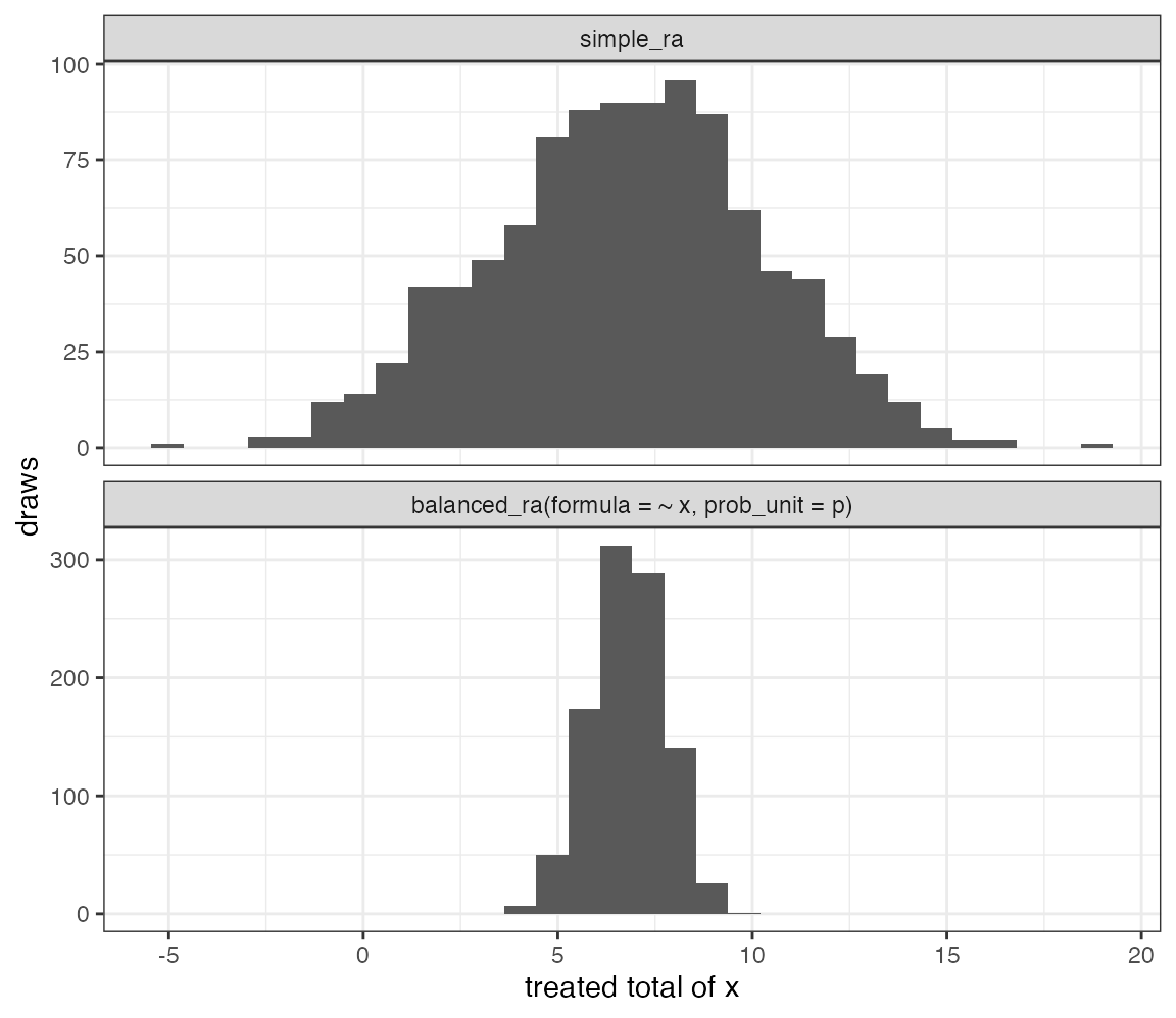

Treated $x$-total under simple_ra and cube-on-X with heterogeneous $p_i$. Cube-on-X is tighter in these draws.

Tightness of $\sum_i x_i Z_i$ is not guaranteed. So buyer beware. Section 3.9 is the warning case: there an assignment exists that would hit the target exactly, and the algorithm never produces it.

What formula balances, and what it does not

We highlight a possible confusion regarding what is balanced in an experimental design.

When you balance a covariate you could have one of two things in mind. The first is that the treated group and the control group should have the same average $x$, so that a simple comparison of their outcomes is not contaminated by a difference in $x$. This is in general a feature that we often hope to gain from randomization. The second is the target the cube method actually pursues: that the treated total of $x$ should come out near $\sum_i x_i p_i$, the total its assignment probabilities imply. When every unit shares the same probability, these two coincide, because splitting the units evenly is the same thing as splitting the column evenly. However when probabilities vary from unit to unit, they come apart.

Here is the intuition. Suppose the units with high $x$ are precisely the ones you decided to treat more often — perhaps $x$ measures need, and you gave the neediest villages the best chance of receiving a program. Then the treated group ought to have the higher mean of $x$. That is not imbalance to be corrected; it is the design you chose. What the cube method does is hold the treated total of $x$ close to the value your own probabilities imply, which leaves the systematic gap in place and squeezes out the draw-to-draw noise around it.

The following makes this concrete with a deliberately extreme case: $p_i$ rising from 0.1 to 0.9 in step with $x$.

set.seed(2)
N2 <- 100
x2 <- sort(rnorm(N2))
p2 <- seq(0.1, 0.9, length.out = N2)   # probability rises with x

gap <- function(Z) mean(x2[Z == 1]) - mean(x2[Z == 0])
g_bal <- replicate(1000, gap(balanced_ra(formula = ~ x2, prob_unit = p2)))
g_sim <- replicate(1000, gap(simple_ra(N = N2, prob_unit = p2)))

rbind(balanced = c(mean_gap = mean(g_bal), sd_gap = sd(g_bal)),
      simple   = c(mean_gap = mean(g_sim), sd_gap = sd(g_sim)))
#>          mean_gap sd_gap
#> balanced     1.06 0.0488
#> simple       1.07 0.1759

The average gap in $x$ between the treated and control groups is large, positive, and essentially the same under both designs. formula did not remove it and was never going to. What formula did was cut the standard deviation of that gap, which is the part that varies from draw to draw.

The practical consequence is that a design with varying $p_i$ needs weighting whatever you pass to formula, exactly as any unequal-probability design does. Section 4 takes that up.

2. Logic

The key idea used in balanced_ra is to randomly switch probability weights between units in ways that shift some into different treatment conditions while satisfying other provided constraints.

For intuition, imagine we have three units who should be assigned to treatment with probability $p = (0.6, 0.7, 0.2)$. The constraint is that the expected treated count is $0.6 + 0.7 + 0.2 = 1.5$. We could imagine various shifts. For instance, shifting $0.3$ from the first unit to the second unit (bringing the second unit to $1$) or $0.4$ from the second unit to the first unit (bringing the first unit to 1). If we randomly choose between these we are effectively randomizing between $p' = (0.3, 1, 0.2)$ and $p'' = (1, 0.3, 0.2)$. If we choose $p'$ with probability $q=\frac{0.4}{0.3+0.4}=\frac{4}{7}$, then $p = qp'+(1-q)p''$, so the unit-level probabilities remain intact. Say in fact that we select $p'' = (1, 0.3, 0.2)$. We might then choose between $(1, 0.5, 0)$ and $(1, 0, 0.5)$; if we do the former with probability $\frac{0.3}{0.3 + 0.2}$, we again keep the unit-level probabilities intact as we move toward a full assignment. At this stage we have one unit in treatment, one unit in control, and one unit to be decided by a coin toss.

The same starting $p$ also admits a three-unit movement, in line with the cube method. A direction $u=(1, -0.5, -0.5)$ has coordinates that sum to $0$, so the treated count is preserved. The largest plus step is $\delta_+=0.4$ and lands at $(1, 0.5, 0)$; the largest minus step is $\delta_-=0.6$ and lands at $(0, 1, 0.5)$. A fair bet takes the plus step with probability $0.6/(0.4+0.6)=0.6$. So here there are more than two units moving, but the martingale idea is the same as in the pair case.

The functions use essentially this logic, now with a broader set of constraints. At each step a direction $u$ is found that respects every constraint still in force, meaning that shifting weight along $u$ leaves each of those constraints exactly where it was. (In the language of linear algebra, $u$ lies in the ‘kernel’ of the constraint matrix.) The randomization is then a fair bet between the two largest steps along $u$, one in each direction, each stopping where the first unit reaches 0 or 1. This stage is the flight.

Sooner or later no such direction remains, and the design has to give something up. That stage is the landing. What it gives up depends on the design. With two arms and no covariates, at most one unit is left fractional and it is settled by a coin. With three or more arms, the walk is allowed to run along a path instead of a closed loop, which lets two arm totals move. With a formula, one column of $X$ is set aside so that a direction exists again — last column first, so that the intercept, and with it the count constraint, is the last thing to go.

Three C++ implementations

balanced_ra uses three C++ implementations, suited to different calls:

Which C++ implementation a call uses.

Call	C++	Does	Paper
balanced_ra(prob_unit = p) or balanced_ra(blocks = b)	cube_two_arm_cpp	Two-arm counts; leftover pairing if blocks	Deville and Tillé (1998), pivotal method
balanced_ra(prob_unit_each = P)	cube_multi_cpp	Three or more arms	Deville and Tillé (2004), cube; Chauvet and Tillé (2006), window
balanced_ra(formula = ~ x)	cube_on_x_cpp	Linear targets on a model matrix $X$	Deville and Tillé (2004), cube; Chauvet and Tillé (2006), window

The three routines are related but not interchangeable. Run the general cube with $X$ equal to the intercept alone and it would reproduce the pivot; run the multi-arm walk with two arms and it would reproduce the pivot too. What the dedicated two-arm routine adds is the leftover pairing described in Section 2.1, and that is why two-arm blocked counts come out tight both inside each block and overall. A generic landing gives up a constraint instead, and would lose one of those two properties.

The listings that follow are lightly abridged from the source. The logic and the arithmetic are as they appear in src/cube.cpp and src/cube_on_x.cpp.

2.1 Two-arm pivot

cube_two_arm_cpp is the pivotal method of Deville and Tillé (1998). The state is a single vector $z$, one running weight per unit, starting at that unit’s probability. Here there is only one constraint, the count, and it forces the direction to be $u = (1, -1)$ on a pair of units still fractional: whatever weight is added to one must be taken from the other, so that $z_i + z_j$ does not move. The randomization is then a fair bet between the two largest steps, one in each direction, each stopping as soon as a unit reaches 0 or 1.

The figures are drawn as networks with units along the bottom and arms along the top. A grey edge marks a unit whose weight is still fractional on that arm but which is not part of the move currently being made. Arrows mark the edges that the move does touch, and they are labelled with the transfer the plus step would make, which is $\delta_+ u$ on that edge, or simply $\pm\delta_+$ whenever $|u_i| = 1$. The number $z$ written under a unit is the weight it currently has on Treat; its weight on Control is $1 - z$.

One draw: four units, target 2.3

We illustrate the logic of the pivot method for a case with four units and heterogeneous probabilities that do not sum to an integer.

Specifically, imagine $p = (0.2, 0.6, 0.7, 0.8)$. These probabilities sum to 2.3, and so every draw should treat 2 or 3 units.

p_piv <- c(0.2, 0.6, 0.7, 0.8)
sum(p_piv)
#> [1] 2.3
balanced_ra(prob_unit = p_piv)
#> [1] 0 1 0 1

Two things in the walk that follows are random, and the illustration fixes both so that there is something definite to look at. The first is the order in which units are visited: balanced_ra() shuffles the units before every draw, precisely so that the answer cannot depend on the order in which you happened to list them, and we suppose here that the shuffle came out as $1, 2, 3, 4$. The second is the outcome of each fair bet, and we suppose that the plus step won every time. At the end one unit is left holding a fractional weight of 0.3, and it is settled by a coin weighted 0.3.

The first pair consists of units 1 and 2. These have a combined mass of $0.8$. The admissible “directions of movement” that keep the sum of probabilities constant is $u=(1,-1,0,0)$. The plus coefficient is $\delta_+=\min(1-0.2,0.6)=0.6$, which assigns unit 2 to control (since $u\delta_+ = (.6, -.6)$ which would yield new position $z' = (0.2, 0.6) + (0.6, -0.6) = (0.8, 0)$). For the negative coefficient we have $\delta_-=\min(0.2,0.4)=0.2$ which assigns unit 1 to control (since the new position would be $z' = (0.2, 0.6) - (0.2, -0.2) = (0, .8)$). We will choose between these two directions, selecting plus with probability $0.2/0.8=1/4$. Note that in this case the question is which gets assigned to control, not which gets assigned to treatment, as it is possible that neither will get assigned to treatment.

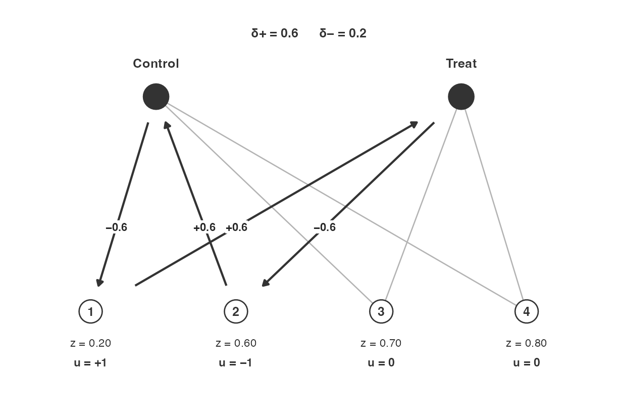
Start. Kernel on units 1 and 2. Arrows are $\delta_+ u$. $\delta_+ = 0.6$ assigns unit 2 to control; $\delta_- = 0.2$ assigns unit 1 to control.

Assume we happened to select the plus coefficient. Then our new $z$ is $z=(0.8,0,0.7,0.8)$. Unit 1 is still open, at $0.8$, and it now pairs with unit 3. And we go again. This time $\delta_+=0.2$ would send unit 1 to 1; $\delta_-=0.3$ would send unit 3 to 1. We choose randomly between these, selecting plus with probability $0.3/0.5=3/5$.

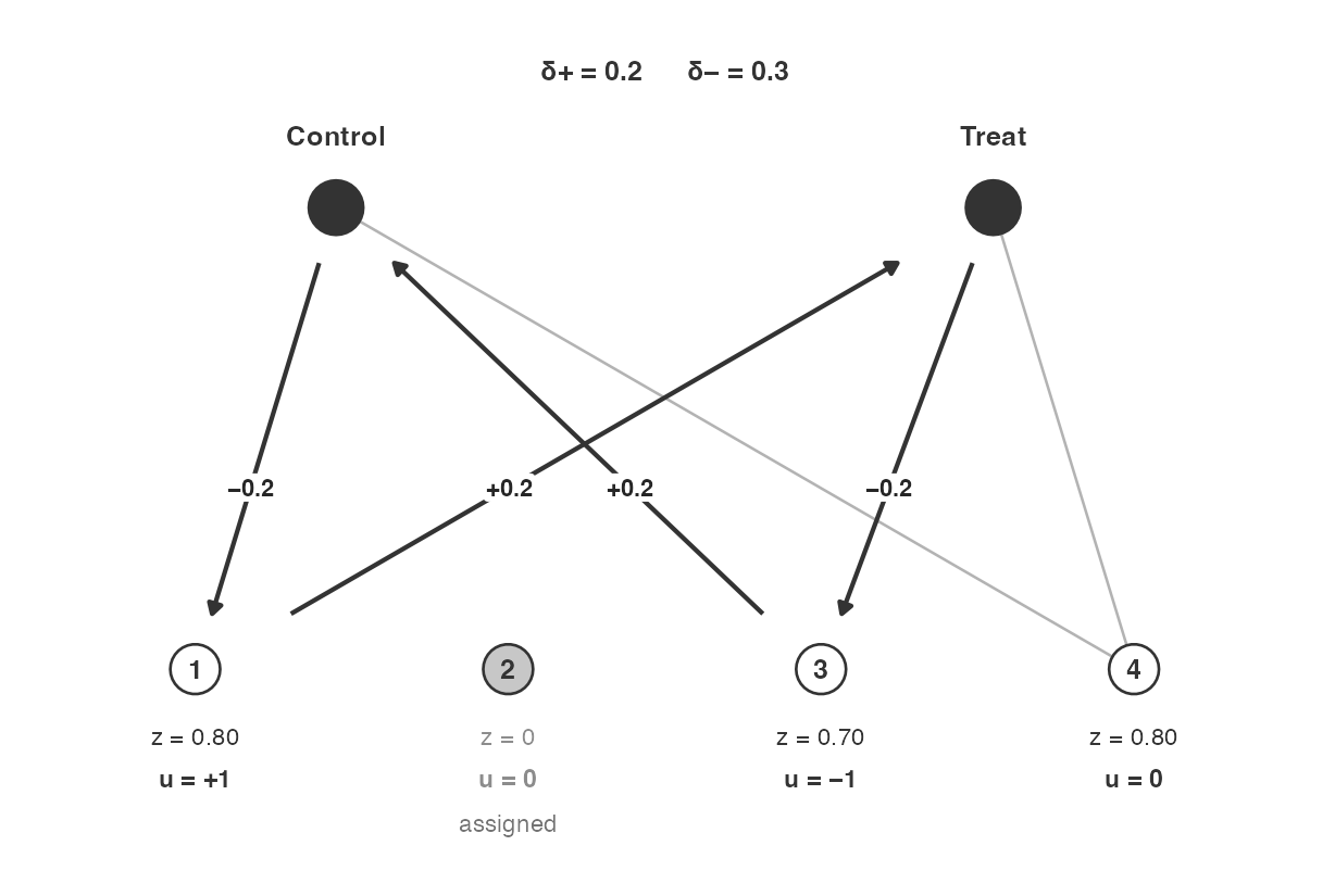
After the first plus step. Unit 2 is assigned. Next pair: units 1 and 3. Arrows are $\delta_+ u$.

Let us imagine again that plus was selected. Then the new $z$ vector is $z=(1,0,0.5,0.8)$. Units 3 and 4 now form a pair. We have possibilities $\delta_+=0.5$, which sends unit 3 to 1 and leaves unit 4 at $0.3$; and $\delta_-=0.2$, which sends unit 4 to 1 and leaves unit 3 at $0.3$. Plus has probability $0.2/0.7=2/7$.

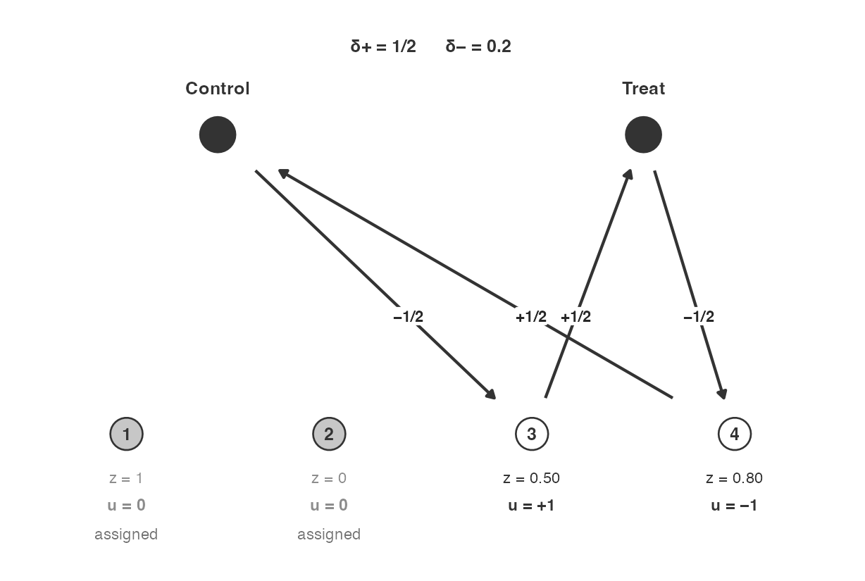
After the second plus step. Units 3 and 4 remain. $\delta_+ = 0.5$ assigns unit 3 (leftover $z_4 = 0.3$); $\delta_- = 0.2$ assigns unit 4.

Assume again we randomly selected plus. Then $z=(1,0,1,0.3)$. One leftover remains, so there is no new pairing possible. We now randomly assign unit 4 with probability $0.3$. The result is that we treat either two or three units.

Leftover pairing across blocks

With blocks, the same pass runs inside each block and leaves at most one fractional unit per block. A second pass then pairs those leftovers as one group, so the overall count stays tight as well. Independent Bernoulli on each block leftover would have kept each block tight and let the overall total wander.

C++: cube_pivot_pass

We see these same steps now in the C++ function:

static void cube_pivot_pass(NumericVector& z, const std::vector<int>& seq,
                            const int* blk, int nb, double tol) {
  std::vector<int> open(nb + 1, -1);
  for (size_t t = 0; t < seq.size(); t++) {
    int j = seq[t];
    // Step 1: skip assigned.
    if (z[j] <= tol || z[j] >= 1.0 - tol) continue;
    int bl = blk[j];
    // Step 2: hold one open unit per block.
    if (open[bl] < 0) { open[bl] = j; continue; }

    // Step 3: kernel pair (z_i + z_j preserved).
    int i = open[bl];
    // Step 4: largest d+ and d-.
    double du = std::min(1.0 - z[i], z[j]);
    double dd = std::min(z[i], 1.0 - z[j]);
    // Step 5: fair bet, then transfer.
    if (unif_rand() < dd / (du + dd)) { z[i] += du; z[j] -= du; }
    else                              { z[i] -= dd; z[j] += dd; }

    // Step 6: housekeeping of open[].
    int keep = (z[i] > tol && z[i] < 1.0 - tol) ? i : j;
    open[bl] = (z[keep] > tol && z[keep] < 1.0 - tol) ? keep : -1;
  }
}

Step	What the line does
1	Units already at 0 or 1 are skipped.
2	The first still-fractional unit in a block is held.
3	A second fractional unit in that block is a pair. The kernel is $(1,-1)$, so $z_i+z_j$ is unchanged.
4	$\delta_+$ and $\delta_-$ are the largest steps that hit 0 or 1.
5	A fair bet: plus with probability $\delta_-/(\delta_++\delta_-)$, then the transfer.
6	The unit that is still fractional stays open; otherwise that block’s slot is empty.

cube_two_arm_cpp then pairs leftovers as if they shared a block, and Bernoulli-rounds any singleton:

  // Step 1: collect leftovers.
  std::vector<int> left;
  for (int t = 0; t < n; t++) {
    int j = seq[t];
    if (z[j] > tol && z[j] < 1.0 - tol) left.push_back(j);
  }
  if (left.size() > 1) {
    // Step 2: fake a single block.
    std::vector<int> one(n, 1);
    // Step 3: same pivot pass (overall count stays tight).
    cube_pivot_pass(z, left, one.data(), 1, tol);
  }
  // Step 4: Bernoulli any singleton leftover.

2.2 Multi-arm cube

With three or more arms a single number per unit is no longer enough to describe where things stand, so the state becomes a table $Z$ with one row per unit and one column per arm. Each row sums to 1, because a unit’s weight has to be spread across the arms somehow, and each column sums to that arm’s target count. cube_multi_cpp is the cube method of Deville and Tillé (2004) run on this table.

The natural picture is a network with the units on one side and the arms on the other, and an edge wherever a cell of $Z$ is still fractional. A move walks along a sequence of edges, adding weight to the first, subtracting from the second, adding to the third, and so on. The alternation is what makes the arithmetic work: two consecutive edges meet at a node, so whatever one takes from that node the other gives back, and the node’s total does not move.

That gives the two stages their concrete meaning here.

• If the walk closes into a loop, or cycle, which is the term the figures below use, every node it visits is entered and left, so every unit’s row total and every arm’s column total survives untouched. This is flight.
• If the walk cannot close and instead runs from one end to another, the two ends are visited only once. Every unit in the middle is fine, and the two arms at the ends are the ones whose totals move. This is landing.

A useful fact makes this tidy. A unit whose row sums to exactly 1 cannot have exactly one fractional cell, since that lone cell would have to make up an integer by itself. So every unit sits on either zero edges or at least two, which means the loose ends of any walk are always arms, never units. Chauvet and Tillé (2006) then supply the trick that makes this fast: rather than searching the whole network, keep a window of just $k$ units with fractional cells.

When blocks are supplied, each block is worked through separately from start to finish, flight and landing together. Within a block the counts therefore come out tight. The overall counts across blocks are a different matter: the leftover pairing that rescues the two-arm case does not extend here, because a block can finish with several fractional units rather than one, and coupling those across blocks could push a within-block arm count more than one away from its target. Section 3.7 shows the overall count wandering as a result.

The figures use the same conventions as Section 2.1: units along the bottom, arms along the top, grey edges for fractional cells that this move does not touch, and arrows labelled with the transfer $\delta_+ u$ that the plus step would make. Under each unit, $z$ is now that unit’s whole row of $Z$, one number per arm, and $u$ is the corresponding row of the direction, which is all zeros if the unit is not on this walk. The two step sizes $\delta_+$ and $\delta_-$ are printed at the top of each figure.

One draw: four units, three arms

P3 <- rbind(
  c(0.2, 0.4, 0.4),
  c(0.4, 0.3, 0.3),
  c(0.6, 0.2, 0.2),
  c(0.8, 0.1, 0.1)
)
P3
#>      [,1] [,2] [,3]
#> [1,]  0.2  0.4  0.4
#> [2,]  0.4  0.3  0.3
#> [3,]  0.6  0.2  0.2
#> [4,]  0.8  0.1  0.1
colSums(P3)
#> [1] 2 1 1
balanced_ra(prob_unit_each = P3, conditions = 1:3)
#> [1] 3 2 1 1

The column targets are $2$, $1$ and $1$. As in Section 2.1 the walk below fixes what is random: the shuffle is supposed to have come out as $1, 2, 3, 4$, so that the first window of $k = 3$ units is units 1, 2 and 3, and the outcome of each bet is stated as we go. Five moves settle the whole table, and because every one of them closes into a loop, no arm total ever moves: the counts finish at exactly $(2, 1, 1)$, which is the target.

The first cycle is a 4-cycle on units 1 and 2, arms 1 and 2. Alternating sign, starting plus on cell $(1,1)$, gives kernel rows $u_1=(+1,-1,0)$, $u_2=(-1,+1,0)$, and $u_3=u_4=(0,0,0)$. The plus coefficient is $\delta_+=\min(1-0.2,0.4,1-0.3,0.4)=\min(0.8,0.4,0.7,0.4)=0.4$, which sends unit 2’s arm-1 cell to 0 and unit 1’s arm-2 cell to 0 (new rows $z_1'=(0.6,0,0.4)$, $z_2'=(0,0.7,0.3)$). The minus coefficient is $\delta_-=\min(0.2,1-0.4,0.3,1-0.4)=\min(0.2,0.6,0.3,0.6)=0.2$, which sends unit 1’s arm-1 cell to 0. Plus with probability $0.2/0.6=1/3$.

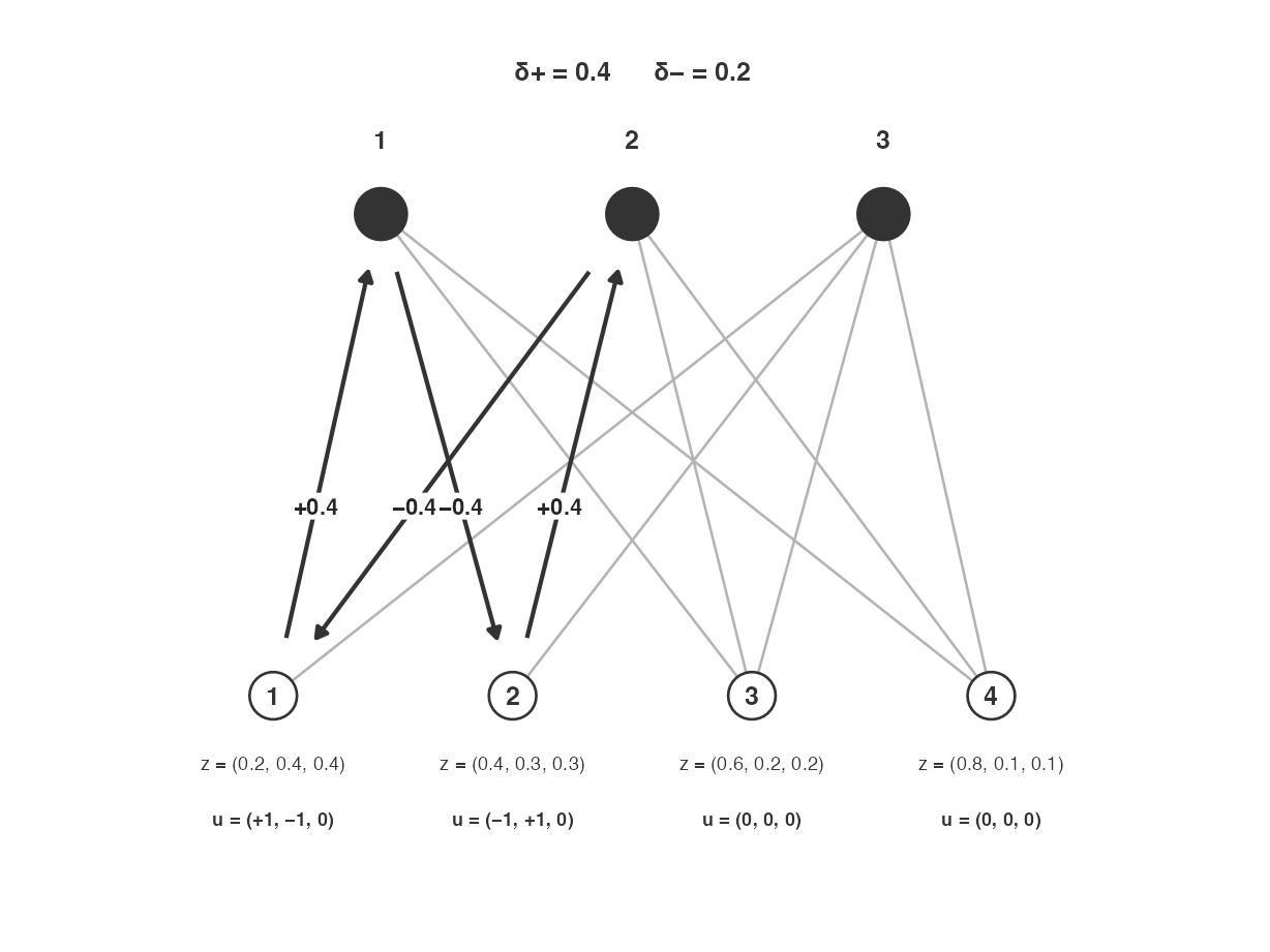
Start. Cycle on units 1–2, arms 1–2. Under each unit, $z$ is the row of $Z$ and $u$ is the kernel row. Arrows are $\delta_+ u$. $\delta_+ = 0.4$ sends unit 2’s arm-1 cell to 0; $\delta_- = 0.2$ sends unit 1’s arm-1 cell to 0.

Assume plus. Then the new rows are $z_1=(0.6,0,0.4)$, $z_2=(0,0.7,0.3)$, $z_3=(0.6,0.2,0.2)$, $z_4=(0.8,0.1,0.1)$. Row and column totals are unchanged. Nobody is fully assigned.

Unit 1 is still open, at $(0.6,0,0.4)$, and now sits in a 6-cycle with units 3 and 2: cells $(1,1)$, $(3,1)$, $(3,2)$, $(2,2)$, $(2,3)$, $(1,3)$. Kernel rows $u_1=(+1,0,-1)$, $u_2=(0,-1,+1)$, $u_3=(-1,+1,0)$, $u_4=(0,0,0)$. $\delta_+=\min(1-0.6,0.6,1-0.2,0.7,1-0.3,0.4)=\min(0.4,0.6,0.8,0.7,0.7,0.4)=0.4$, which assigns unit 1 to arm 1. $\delta_-=\min(0.6,1-0.6,0.2,1-0.7,0.3,1-0.4)=\min(0.6,0.4,0.2,0.3,0.3,0.6)=0.2$, which sends unit 3’s arm-2 cell to 0. Plus with probability $0.2/0.6=1/3$.

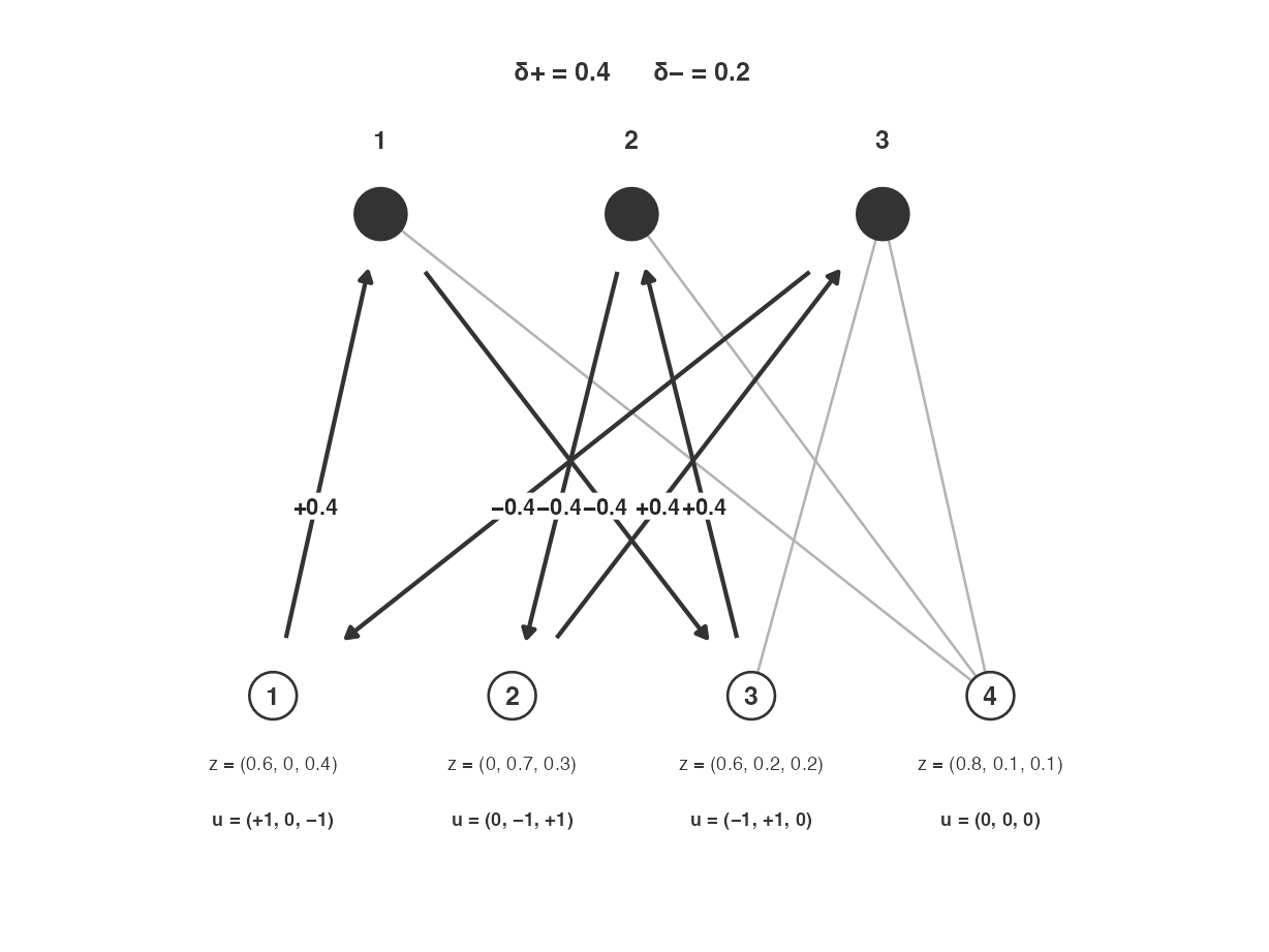
After the first plus step. Next cycle on units 1, 3, 2. $\delta_+ = 0.4$ assigns unit 1 to arm 1; $\delta_- = 0.2$ sends unit 3’s arm-2 cell to 0.

Assume plus. Then $z_1=(1,0,0)$, $z_2=(0,0.3,0.7)$, $z_3=(0.2,0.6,0.2)$, $z_4=(0.8,0.1,0.1)$. Unit 1 is assigned.

Units 3 and 4 now form a 4-cycle on arms 2 and 1: cells $(3,2)$, $(3,1)$, $(4,1)$, $(4,2)$. Kernel rows $u_3=(-1,+1,0)$, $u_4=(+1,-1,0)$, and $u_1=u_2=(0,0,0)$. $\delta_+=\min(1-0.6,0.2,1-0.8,0.1)=\min(0.4,0.2,0.2,0.1)=0.1$, which sends unit 4’s arm-2 cell to 0. $\delta_-=\min(0.6,1-0.2,0.8,1-0.1)=\min(0.6,0.8,0.8,0.9)=0.6$, which sends unit 3’s arm-2 cell to 0. Plus with probability $0.6/0.7=6/7$.

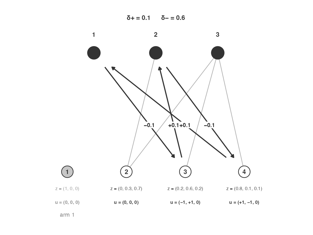
After the second plus step. Unit 1 is assigned. Cycle brings in unit 4. $\delta_+ = 0.1$ sends unit 4’s arm-2 cell to 0; $\delta_- = 0.6$ sends unit 3’s arm-2 cell to 0.

Assume plus. Then $z_1=(1,0,0)$, $z_2=(0,0.3,0.7)$, $z_3=(0.1,0.7,0.2)$, $z_4=(0.9,0,0.1)$.

A 6-cycle on units 2, 3, and 4: cells $(2,2)$, $(3,2)$, $(3,1)$, $(4,1)$, $(4,3)$, $(2,3)$. Kernel rows $u_2=(0,+1,-1)$, $u_3=(+1,-1,0)$, $u_4=(-1,0,+1)$, and $u_1=(0,0,0)$. $\delta_+=\min(1-0.3,0.7,1-0.1,0.9,1-0.1,0.7)=\min(0.7,0.7,0.9,0.9,0.9,0.7)=0.7$, which assigns unit 2 to arm 2. $\delta_-=\min(0.3,1-0.7,0.1,1-0.9,0.1,1-0.7)=\min(0.3,0.3,0.1,0.1,0.1,0.3)=0.1$, which assigns unit 4 to arm 1. Plus with probability $0.1/0.8=1/8$.

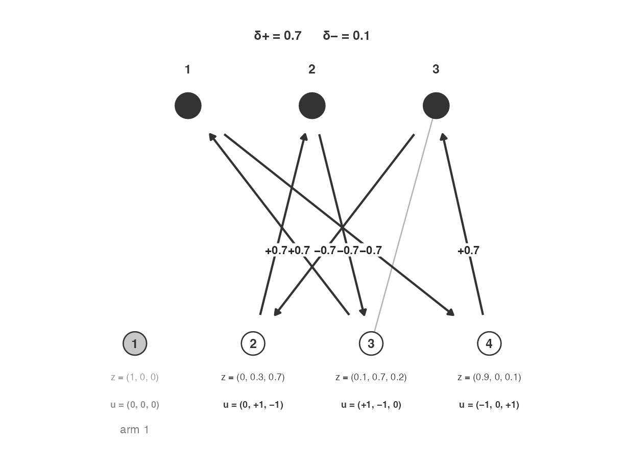
After the third plus step. Cycle on units 2, 3, 4. $\delta_+ = 0.7$ assigns unit 2 to arm 2; $\delta_- = 0.1$ assigns unit 4 to arm 1.

Minus is selected this time. Then $z_1=(1,0,0)$, $z_2=(0,0.2,0.8)$, $z_3=(0,0.8,0.2)$, $z_4=(1,0,0)$. Units 1 and 4 are both settled on arm 1, and what remains is a single loop on units 2 and 3 over arms 2 and 3.

That last loop (not shown) finishes the draw. The cells are $(2,2)$, $(3,2)$, $(3,3)$, $(2,3)$ holding $0.2$, $0.8$, $0.2$, $0.8$, so $\delta_+ = \min(0.8, 0.8, 0.8, 0.8) = 0.8$ and $\delta_- = \min(0.2, 0.2, 0.2, 0.2) = 0.2$, and plus is taken with probability $0.2/1.0$. Whichever way the bet falls, one of the two units goes to arm 2 and the other to arm 3. Adding up: unit 1 and unit 4 on arm 1, and units 2 and 3 splitting arms 2 and 3 between them. The counts are $(2, 1, 1)$, which is what the column totals asked for.

C++: the fair bet, the window, and per-block landing

Three routines do the work. cube_move takes the bet along a walk that has already been found, cube_step finds the walk (that part is left to the source, since it is graph bookkeeping rather than design logic), and cube_process decides which units to look at.

cube_move is the direct counterpart of Section 2.1’s fair bet, with the alternating sign that makes consecutive cells cancel at the node they share.

static void cube_move(std::vector<double>& Z, int n,
                      const std::vector<int>& cu, const std::vector<int>& ca,
                      double tol) {
  int m = cu.size();
  double dplus = R_PosInf, dminus = R_PosInf;
  // Step 1: largest d+ and d- (alternating sign).
  for (int e = 0; e < m; e++) {
    double z = Z[cu[e] + (size_t) ca[e] * n];
    if (e % 2 == 0) { dplus = std::min(dplus, 1.0 - z); dminus = std::min(dminus, z); }
    else            { dplus = std::min(dplus, z); dminus = std::min(dminus, 1.0 - z); }
  }
  if (!R_FINITE(dplus + dminus) || dplus + dminus <= 0) return;

  // Step 2: fair bet.
  bool up = unif_rand() < dminus / (dplus + dminus);
  // Step 3: apply the transfer.
  for (int e = 0; e < m; e++) {
    size_t ix = cu[e] + (size_t) ca[e] * n;
    double s = (e % 2 == 0) ? 1.0 : -1.0;
    Z[ix] += up ? s * dplus : -s * dminus;
    if (Z[ix] < tol) Z[ix] = 0.0;
    if (Z[ix] > 1.0 - tol) Z[ix] = 1.0;
  }
}

Step	What the line does
1	Walk the cycle with alternating sign. $\delta_+$ and $\delta_-$ are the largest steps that hit 0 or 1 on any cell of the walk.
2	A fair bet: plus with probability $\delta_-/(\delta_++\delta_-)$.
3	Add $+\delta_+$ or $-\delta_-$ times the sign of each edge. Row totals and interior column totals do not move.

cube_process is the Chauvet–Tillé window. It holds at most $k$ units at a time, keeps only those with at least two fractional cells, and refills the window from a list as units settle. Because a window of $k$ such units always contains a loop, this is enough: there is no need to look at the rest.

static void cube_process(std::vector<double>& Z, int n, int k,
                         const std::vector<int>& units, double tol,
                         CubeWork& ws, bool allow_path) {
  size_t ptr = 0;
  std::vector<int> W;                       // the window
  W.reserve(k);
  // Step 1: a bound on the number of moves, so a numerical oddity cannot
  // turn into an infinite loop. Every real move settles at least one cell.
  long long guard = (long long) units.size() * k + 10;
  while (guard-- > 0) {
    // Step 2: top the window up to k units. A unit with fewer than two
    // fractional cells has nothing left to trade, so it is passed over.
    while ((int) W.size() < k && ptr < units.size()) {
      int u = units[ptr++];
      if (cube_nfrac(Z, n, k, u, tol) >= 2) W.push_back(u);
    }
    if (W.empty()) break;
    // Step 3: one move on the window. cube_step finds a loop if the window
    // has one and takes cube_move along it; if it has none and paths are
    // allowed, it lands along a path instead. False means nothing is left.
    if (!cube_step(Z, n, k, W, tol, ws, allow_path)) break;
    // Step 4: drop whatever the move settled, then go round again.
    std::vector<int> keep;
    for (size_t t = 0; t < W.size(); t++) {
      if (cube_nfrac(Z, n, k, W[t], tol) >= 2) keep.push_back(W[t]);
    }
    W.swap(keep);
  }
}

Step	What the line does
1	An upper bound on the loop. Each move settles at least one of the $N k$ cells, so a correct run finishes well inside the bound; the guard exists only so that a floating-point surprise cannot hang the draw.
2	Fill the window to $k$ units, skipping any unit with fewer than two fractional cells, since such a unit has already been decided.
3	Make one move. A loop is preferred and leaves every total intact; a path is used only when no loop exists, and only when allow_path says landing is permitted.
4	Units that the move settled leave the window and their places are refilled at Step 2.

cube_multi_cpp then calls this once per block, with allow_path = true so that each block flies and lands on its own:

  // Two-arm leftover coupling does not extend. Each block is landed on
  // its own. Overall tightness may slip when several remainders land
  // the same way.
  for (int bl = 1; bl <= nb; bl++)
    cube_process(Z, n, k, bu[bl], tol, ws, true);

That loop is the whole reason for the caveat in Section 3.7. Every block is handled in isolation, so every block comes out tight, and nothing in the code arranges for one block’s rounding to compensate for another’s.

2.3 Cube-on-X

The third routine, cube_on_x_cpp, runs the cube method on the balancing matrix $X$ that formula supplies. It handles two arms and does not accept blocks. Under ~ x the matrix has two columns, and each is a constraint: the intercept column asks the sum of the weights to stay put, which is the count constraint, and the $x$ column asks the weighted total of $x$ to stay put, which is the covariate constraint.

A move may only go in a direction $u$ that leaves both columns undisturbed, which written out means $X'u = 0$ — for the intercept column, $\sum_i u_i = 0$, and for the $x$ column, $\sum_i x_i u_i = 0$. With $q$ columns the routine takes a window of $q + 1$ units, since $q$ constraints on $q + 1$ unknowns always leave at least one direction free. So under ~ x the window has three units. When landing is reached the routine reduces $q$ by one, dropping the last column of $X$ first, until a direction exists again; the intercept, and with it the count, is therefore the last constraint to be given up.

Compare with the pivot approach. The pivot’s move takes weight from one unit and gives it to another, $u = (1, -1)$ on a pair. That leaves the count alone, since the two changes cancel, but it moves the total of $x$ by $x_i - x_j$, which is zero only if the pair so happens to share a value of $x$. Holding both constraints at once needs at least three units, which is exactly why the window is $q + 1$ rather than 2.

One further detail matters for reading Section 3.9. Units are sorted by the first column of $X$ that is not constant — usually the covariate, since an intercept is constant — and a coin flip then decides whether to read that order forwards or backwards. The sort is a choice made in this implementation rather than a requirement of the cube method, and it is there so that landing is left with units whose covariate values are close together. The walk below assumes increasing $x$ and no reversal.

One draw: $x=(1,2,3,6)$, $p_i=1/2$

Start at $z=(1/2,1/2,1/2,1/2)$. The window is units 1, 2, and 3. The kernel direction (up to scale) is $u=(1,-2,1,0)$: $1-2+1=0$ and $1\cdot 1+2\cdot(-2)+3\cdot 1=0$. Both maximal steps have size $\delta_+=\delta_-=1/4$. Plus assigns unit 2 to control; minus assigns unit 2 to treatment. Plus with probability $(1/4)/(1/4+1/4)=1/2$.

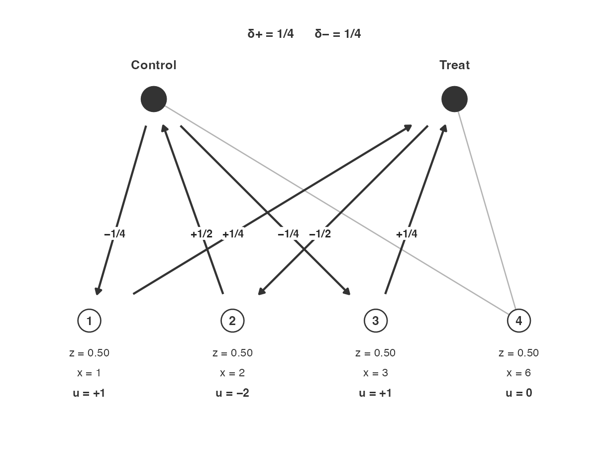
Start. Window of three units. Kernel $u = (1, -2, 1, 0)$. Arrows are $\delta_+ u$; unit 2 moves twice as far. $\delta_\pm = 1/4$.

Assume plus. Then $z=(0.75,0,0.75,0.5)$. Sum $z$ is still 2; the treated $x$-total is still 6. The next window is the three open units. An admissible $u$ is $(3,0,-5,2)$: $3-5+2=0$ and $1\cdot 3+3\cdot(-5)+6\cdot 2=0$. $\delta_+=1/12$ assigns unit 1 to treatment; $\delta_-=1/20$ assigns unit 3 to treatment. Plus with probability $(1/20)/(1/12+1/20)=3/8$. Neither of these two steps sends a unit to 0.

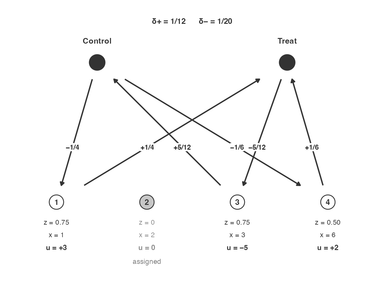
After the first plus step. Unit 2 is assigned. Arrows are $\delta_+ u$ with $u = (3, 0, -5, 2)$. $\delta_+ = 1/12$; $\delta_- = 1/20$.

Assume plus. Then $z=(1,0,1/3,2/3)$. Only units 3 and 4 are still fractional, and there are two constraints for them to satisfy, which is one too many: two equations on two unknowns leave no freedom at all, so no direction remains. The only move available on a pair is to take from one and give to the other, which keeps the count but shifts the $x$-total by $x_3 - x_4$. The algorithm therefore gives up the $x$ column.

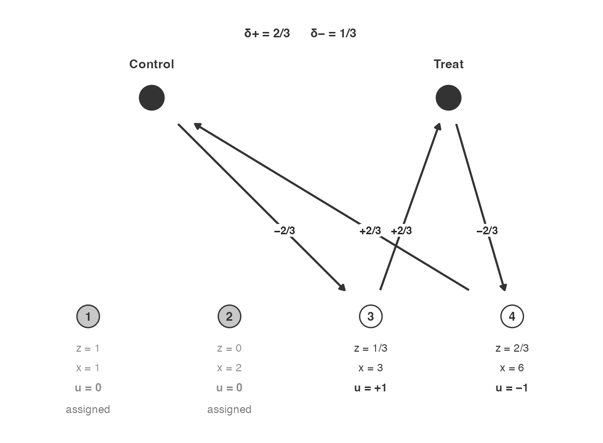
After $\delta_+ = 1/12$. No kernel remains on both columns, so $x$ is dropped. Arrows are the count-only landing move $\delta_+ u$. $\delta_+ = 2/3$; $\delta_- = 1/3$.

What remains is the count constraint alone, and the direction $u=(0,0,1,-1)$. $\delta_+=2/3$ assigns unit 3 to treatment and unit 4 to control, for a treated $x$-total of $4$; $\delta_-=1/3$ does the reverse, for a total of $7$. Plus with probability $(1/3)/(2/3+1/3)=1/3$. Neither hits the target of $6$.

In this particular example nothing better was available: with $x = (1,2,3,6)$ and two units treated, the attainable totals are $3, 4, 5, 7, 8$ and $9$, and $6$ is simply not among them. So landing did what it could but couldn’t do the impossible. That is not always the reason a target is missed, though, and the two sections that close Section 3 are the cases where a perfectly attainable target is missed anyway — Section 3.8 because the flight can stop at a fractional point from which no exact assignment is reachable, and Section 3.9 because the narrow window can commit to a direction that rules the exact assignments out.

C++: the main loop

Here is how the code works. At any point the loop takes the next $q + 1$ units off the front of a queue, asks for a direction, and moves along it. Only if no direction can be found—first on the small window, then on every unit still fractional—does it give up a column.

    // Step 1: the window is the first q+1 units still fractional.
    int w = std::min(nf, q_use + 1);
    std::vector<int> W(queue.begin() + head, queue.begin() + head + w);
    // Step 2: find a direction on that window and step along it.
    bool moved = try_window(z, W, Xs, n, q_use, A, u, tol);
    // Step 3: a small window can fail even when a direction exists on the
    // whole remainder, so try every remaining unit before giving anything up.
    if (!moved && w < nf) {
      std::vector<int> Wall(queue.begin() + head, queue.end());
      moved = try_window(z, Wall, Xs, n, q_use, A, u, tol);
      if (moved) { W.swap(Wall); w = nf; }
    }
    // Step 4: still nothing. Drop the last column of X and try again. The
    // intercept is column 0, so the count constraint goes last of all.
    if (!moved) {
      q_use--;
      continue;
    }
    // Step 5: the window's units are sent to the back of the queue, and
    // those that settled do not go back on it at all.
    head += w;
    for (int t = 0; t < w; t++) {
      int i = W[t];
      if (z[i] > tol && z[i] < 1.0 - tol) queue.push_back(i);
    }

try_window builds the little matrix $X'$ restricted to the window, hands it to kernel_vector for a direction, and then takes the same fair bet as the pivot did, now applied to every unit with $u_i \neq 0$ rather than to just two.

C++: finding a direction

kernel_vector is where “a direction that respects the constraints” becomes arithmetic. It is ordinary Gaussian elimination: reduce the constraint matrix, and any column that did not end up as a pivot is a coordinate you are free to choose, from which the pivot coordinates follow.

// Find u != 0 with A u = 0, where A is X' restricted to the window:
// q constraints (rows) across w units (columns).
static bool kernel_vector(const std::vector<double>& A, int q, int w,
                          std::vector<double>& u, double eps) {
  if (w < 1) return false;
  u.assign(w, 0.0);
  // Step 1: no constraints left at all, so anything goes. Take from one
  // unit and give to another, which is the pivot move of Section 2.1.
  if (q < 1) {
    if (w == 1) return false;
    u[0] = 1.0; u[1] = -1.0;
    return true;
  }

  // Step 2: row-reduce A, choosing the largest available entry as each
  // pivot so that the arithmetic stays well conditioned. Columns that
  // never become pivots are the free ones.
  std::vector<double> M = A;
  /* ... elimination, recording is_piv[] and piv_col[] ... */

  std::vector<int> free_cols;
  for (int c = 0; c < w; c++) if (!is_piv[c]) free_cols.push_back(c);
  // Step 3: no free column means no direction. The caller widens the
  // window, or drops a constraint.
  if (free_cols.empty()) return false;

  // Step 4: pick one free column at random, set it to 1, and solve for
  // the pivot coordinates. This is the direction.
  int idx = (int) std::floor(unif_rand() * (double) free_cols.size());
  int jf = free_cols[idx];
  u[jf] = 1.0;
  /* ... back-substitute for the pivot coordinates ... */

  // Step 5: rescale to a sensible size, then check that A u really is
  // zero. A direction that fails this test is refused rather than used.
  double nrm = 0.0, resid = 0.0;
  for (int j = 0; j < w; j++) nrm = std::max(nrm, std::fabs(u[j]));
  if (nrm < eps) return false;
  for (int j = 0; j < w; j++) u[j] /= nrm;
  for (int r = 0; r < q; r++) {
    double au = 0.0;
    for (int j = 0; j < w; j++) au += A[(size_t) r * w + j] * u[j];
    resid = std::max(resid, std::fabs(au));
  }
  return resid < 1e-5;
}

Step	What the line does
1	With nothing left to respect, take weight from one unit and give it to another. This is landing at its last extremity, and it is the pivot move.
2	Row-reduce the constraints. Partial pivoting, meaning the largest entry is used at each stage, keeps the result stable when the covariate is on an awkward scale.
3	If every column is a pivot, the constraints pin the window down completely and there is no direction to take. The caller responds by widening the window and then, failing that, by dropping a column.
4	Choose a free column, set that coordinate to 1, and solve for the rest.
5	Rescale, then verify. The direction is only accepted if it really does leave every constraint where it was.

Step 4 deserves a sentence, because it is the one place where the implementation makes a choice that the cube method leaves open. When more than one free column exists the kernel has more than one dimension, and there are infinitely many valid directions to choose from. The routine picks uniformly among the coordinate directions that Gaussian elimination happens to produce, which is not the same as choosing uniformly among all valid directions, and which of them appear depends on the pivoting order. Every one of them is a legitimate direction, so each unit’s probability is exact whichever is drawn. But which balanced assignments are reachable, and with what frequency, does depend on this choice. Section 3.9 is a case where a one-dimensional kernel leaves no choice at all, and the single available direction rules out the assignments that would have hit the target exactly.

3. Examples

We provide next a set of examples of balanced_ra in action. Each example draws an assignment and then checks a claim about it. A green tick means the claim held on the draws shown (a check that fails stops the vignette from building, so a tick you can see is a tick that was earned when this page was made). Sections 3.7, 3.8 and 3.9 are different: they carry a red cross, and they are there to mark claims that are not guaranteed and that in fact fail.

3.1 One winner from unequal chances

Four contestants have winning probabilities 0.50, 0.30, 0.15 and 0.05. The probabilities sum to 1, so exactly one contestant should win each time. Neither of the obvious alternatives manages this: simple_ra() would honour the four chances but would sometimes crown two winners and sometimes none, and complete_ra() would crown exactly one but would require all four have an equal chance of being that one.

Two things are therefore worth checking here, and the example checks both: that every draw has exactly one winner, and that each contestant wins at close to the rate asked for. The second of these is a statement about a long run of draws rather than about any one of them, so we take a hundred thousand draws. A draw of four units is cheap enough that this costs a few seconds.

chances <- c(0.5, 0.3, 0.15, 0.05)
n_race <- 100000
set.seed(1)
which(balanced_ra(prob_unit = chances) == 1)
#> [1] 4
Z_race <- replicate(n_race, balanced_ra(prob_unit = chances))
win_rate <- rowMeans(Z_race)
race <- rbind(chance = chances, win_rate = win_rate)
colnames(race) <- paste0("contestant ", seq_along(chances))
race
#>          contestant 1 contestant 2 contestant 3 contestant 4
#> chance          0.500          0.3         0.15       0.0500
#> win_rate        0.501          0.3         0.15       0.0492

✓ Every draw has exactly one winner.

✓ Each contestant’s win rate tracks the chance supplied (max absolute gap below 0.02).

3.2 Two-arm counts with blocks

Ten blocks of three units, equal probabilities. The overall target is 15. Each block’s target is 1.5, so each block should contribute 1 or 2 treated units, and the total should be 15 on every draw.

set.seed(12)
blocks10 <- rep(1:10, each = 3)
balanced_ra(blocks = blocks10)
#>  [1] 0 1 0 0 1 0 1 0 1 1 0 0 1 0 0 1 1 0 0 1 1 0 1 1 1 0 1 0 1 0
r_blk <- replicate(2000, balanced_ra(blocks = blocks10))
table(colSums(r_blk))
#> 
#>   15 
#> 2000
block_range <- sapply(1:10, function(b)
  range(colSums(r_blk[blocks10 == b, , drop = FALSE])))
rownames(block_range) <- c("min", "max")
block_range
#>     [,1] [,2] [,3] [,4] [,5] [,6] [,7] [,8] [,9] [,10]
#> min    1    1    1    1    1    1    1    1    1     1
#> max    2    2    2    2    2    2    2    2    2     2

✓ Every draw treats 15 units, and every block contributes 1 or 2.

3.3 Three arms, no blocks

Arm 2 has expected count $1.13$, so a tight assignment gives that arm 1 or 2 units every time.

P23 <- cbind(c(0.15, 0.47), c(0.65, 0.48), c(0.20, 0.05))
P23
#>      [,1] [,2] [,3]
#> [1,] 0.15 0.65 0.20
#> [2,] 0.47 0.48 0.05
colSums(P23)
#> [1] 0.62 1.13 0.25
set.seed(4)
balanced_ra(prob_unit_each = P23, conditions = 1:3)
#> [1] 3 2
Z23 <- replicate(2000, 
  balanced_ra(prob_unit_each = P23, conditions = 1:3))
table(colSums(Z23 == 2))
#> 
#>    1    2 
#> 1714  286

✓ Arm 2 receives 1 or 2 units on every draw.

3.4 Heterogeneous probabilities

Eighty units, five blocks of uneven size, probabilities drawn from the unit interval. Unit-level means should track $p$.

set.seed(3)
n <- 80
p <- runif(n)
blocks_h <- sample(1:5, n, replace = TRUE, prob = 1:5)
reps_h <- replicate(2000, balanced_ra(prob_unit = p, blocks = blocks_h))
share <- rowMeans(reps_h)
ggplot(data.frame(p, share), aes(p, share)) +
  geom_abline(slope = 1, intercept = 0, colour = "grey40") +
  geom_point(size = 1.5) +
  coord_equal(xlim = c(0, 1), ylim = c(0, 1), expand = FALSE) +
  labs(x = "supplied probability", y = "share treated") +
  theme_bw(base_size = 11) +
  theme(panel.grid.minor = element_blank())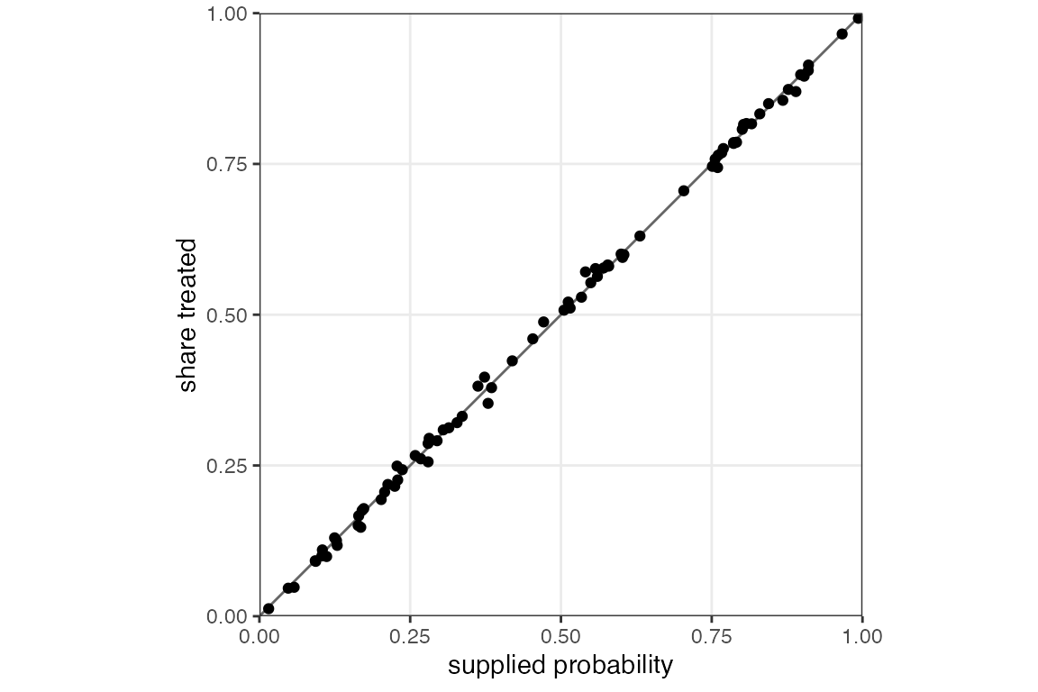

✓ Unit-level shares track the supplied probabilities (max absolute gap below 0.08).

3.5 Clusters

When whole clusters are assigned together, the design has one decision per cluster rather than one per unit, and the count that is held tight becomes a count of clusters. That is true whatever the clusters’ sizes, so the number of treated units is free to vary as long as the clusters differ in size.

Six clusters of unequal size, with cluster probabilities that sum to 3, so three clusters should be treated on every draw.

set.seed(8)
clusters <- rep(1:6, times = c(3, 1, 4, 2, 5, 3))
p_cluster <- c(0.2, 0.4, 0.6, 0.8, 0.5, 0.5)
z_cl <- balanced_ra(prob_unit = p_cluster[clusters], clusters = clusters)
table(clusters, z_cl)
#>         z_cl
#> clusters 0 1
#>        1 3 0
#>        2 1 0
#>        3 0 4
#>        4 0 2
#>        5 0 5
#>        6 3 0

✓ Units in a cluster share an assignment, and exactly three clusters are treated on every draw.

Clusters with a covariate

clusters and formula can be combined. If you do this, each cluster is collapsed to a single row that stands in for it. Its probability is the probability its units share, and its covariates are the averages of its units’ covariates. That is what makes a cluster behave like a unit: the intercept column of a model matrix is a column of ones, and averaging a column of ones leaves a column of ones, so the count constraint still reads “how many clusters are treated”. Under formula = ~ x the balanced quantity is correspondingly the total across treated clusters of each cluster’s mean of x, with every cluster counting once however many units it holds.

An alternative would have been to add the covariates up rather than average them, which would have turned the intercept column into cluster sizes and the count constraint into “how many units are treated”, leaving the number of treated clusters free to wander.

set.seed(19)
clusters <- rep(1:6, times = c(3, 1, 4, 2, 5, 3))
x_cl <- c(-2, -1, 0, 1, 2, 3)[clusters]
Z_clx <- replicate(2000, balanced_ra(prob_unit = p_cluster[clusters],
                                     clusters = clusters, formula = ~ x_cl))
n_treated_clx <- apply(Z_clx, 2, function(z)
  sum(tapply(z, clusters, function(v) v[1])))
table(treated_clusters = n_treated_clx)
#> treated_clusters
#>    3 
#> 2000
table(treated_units = colSums(Z_clx))
#> treated_units
#>   6   7   8   9  10  11  12 
#> 265 106 310 602 253 222 242

✓ With formula and clusters together, exactly three clusters are treated on every draw, and no cluster is split.

However, the number of treated units varies because the clusters have different sizes. The number of treated clusters does not.

3.6 formula plus blocks

Balancing on a covariate does not accept blocks. A block factor in the formula is a column of $X$, not the blocks argument. The call is refused rather than approximated, since the two devices would be pulling in different directions.

x_fb <- c(1, 2, 3, 6)
blocks_fb <- rep(1:2, each = 2)
balanced_ra(formula = ~ x_fb, blocks = blocks_fb)
#> Error:
#> ! `formula` and `blocks` cannot both be set. Use the formula or use `blocks`, but not both.

✓ formula plus blocks is refused.

That is one for the future.

3.7 Multi-arm totals with blocks are not tight

Overall tightness is not guaranteed with three or more arms and blocks. The within-block counts stay tight, as always, but the counts added up across blocks can drift, because the leftover pairing that rescues the two-arm case does not extend to more arms. The loop shown at the end of Section 2.2 is the reason: each block is worked through on its own, and nothing arranges for one block’s rounding to offset another’s.

Three blocks of two units, three arms, and every probability equal to $1/3$. Each block should give each arm 0 or 1 unit, since a block only has two units to give. The overall target is 2 units per arm, but the overall count can come out anywhere from 0 to 3.

set.seed(16)
P_mb <- matrix(1 / 3, 6, 3)
blocks_mb <- rep(1:3, each = 2)
balanced_ra(prob_unit_each = P_mb, blocks = blocks_mb, conditions = 1:3)
#> [1] 2 1 1 2 1 2
Z_mb <- replicate(2000, 
  balanced_ra(prob_unit_each = P_mb, blocks = blocks_mb, conditions = 1:3))
table(colSums(Z_mb == 1))
#> 
#>   0   1   2   3 
#>  90 465 848 597

✓ Within each block, each arm’s count is 0 or 1.

✗ Overall arm counts are always the floor or the ceiling of the overall target (here, always 2).

The red cross is the point of the example. Do not read overall floor-or-ceiling tightness off a blocked multi-arm design; check it, or use two arms, where the guarantee does hold.

3.8 An attainable covariate total that is still missed

Flight stops as soon as no direction respects every constraint. The point it stops at satisfies all the constraints, but it need not be an assignment: some units can still be holding fractional weights. Landing then has to give a constraint up, and once it does, an exactly balanced assignment can be out of reach even though one existed at the outset.

Consider four units with covariate $x = (1, 2, 3, 4)$ and $p_i = 1/2$ throughout, so that two units are treated on every draw. The target treated total of $x$ is $5$, and two assignments attain it exactly: treat units 1 and 4, or treat units 2 and 3.

complete_ra(N = 4, m = 2) spreads its draws evenly over all six pairs, so those two attaining assignments get a third of the mass between them. balanced_ra(formula = ~ x) gives them less than that — about a quarter — and puts the surplus on the pairs whose totals are 4 and 6, one either side of the target.

x <- c(1, 2, 3, 4)
pairs <- combn(4, 2)
n_draw <- 8000
set.seed(20260822)
Z_complete <- replicate(n_draw, complete_ra(N = 4, m = 2))
Z_balanced <- replicate(n_draw, balanced_ra(formula = ~ x))

tab <- data.frame(
  treated = apply(pairs, 2, paste, collapse = ","),
  `x treated` = apply(pairs, 2, function(j) paste(x[j], collapse = ",")),
  `sum x` = apply(pairs, 2, function(j) sum(x[j])),
  complete = 1 / 6,
  balanced = vertex_share(Z_balanced),
  check.names = FALSE
)
knitr::kable(tab, digits = 3,
             caption = "Shares of the six assignments of two treated units with $x = (1, 2, 3, 4)$. The target pair-sum is 5 and is attained by treating units 1 and 4 or units 2 and 3. `balanced_ra` does not concentrate on those two.")

Shares of the six assignments of two treated units with $x = (1, 2, 3, 4)$. The target pair-sum is 5 and is attained by treating units 1 and 4 or units 2 and 3. balanced_ra does not concentrate on those two.

treated	x treated	sum x	complete	balanced
1,2	1,2	3	0.167	0.121
1,3	1,3	4	0.167	0.255
1,4	1,4	5	0.167	0.126
2,3	2,3	5	0.167	0.126
2,4	2,4	6	0.167	0.251
3,4	3,4	7	0.167	0.122

rbind(
  complete = c(p = mean(Z_complete), treated = mean(colSums(Z_complete))),
  balanced = c(p = mean(Z_balanced), treated = mean(colSums(Z_balanced)))
)
#>            p treated
#> complete 0.5       2
#> balanced 0.5       2

set.seed(31)
Z_simple <- replicate(n_draw, simple_ra(N = 4, prob = 0.5))
sx_complete <- colSums(x * Z_complete)
sx_balanced <- colSums(x * Z_balanced)
sx_simple   <- colSums(x * Z_simple)
rbind(
  simple   = c(mean = mean(sx_simple),   var = var(sx_simple)),
  complete = c(mean = mean(sx_complete), var = var(sx_complete)),
  balanced = c(mean = mean(sx_balanced), var = var(sx_balanced))
)
#>          mean  var
#> simple   4.95 7.47
#> complete 5.01 1.70
#> balanced 5.00 1.47

We see that balanced_ra(formula = ~ x) is the best of the three here, comfortably better than simple_ra() and a little better than complete_ra() in terms of variance reduction. The failure being demonstrated is not that “the design does not help”; it is that the design does not deliver the exact target even when the exact target is attainable, and so cannot always be relied on to do so.¹

✓ First-order probabilities remain 1/2, and every draw treats exactly two units.

✗ The treated x-total is 5 on every draw.

3.9 An example of an attainable covariate total that never appears at all

Section 3.8 missed the target often. This example misses it always, and the reason sits earlier in the algorithm.

Take four units with $x = (1, 2, 2, 3)$ and $p_i = 1/2$, so two units are treated and the target treated total of $x$ is $\sum_i x_i p_i = 4$. Two assignments attain it exactly: treat the two 2’s, or treat the 1 and the 3. But it turns out that neither of these profiles is ever drawn.

x <- c(1, 2, 2, 3)
set.seed(20260822)
Z <- replicate(1000, balanced_ra(formula = ~ x))
sx <- colSums(x * Z)
table(sx)
#> sx
#>   3   5 
#> 509 491

✓ First-order probabilities remain 1/2, and every draw treats exactly two units.

✗ The treated x-total is 4 on every draw.

Unlike Section 3.8, this is not landing coming as close as it can. The damage is done during flight, by the narrow window.

The window here holds $q + 1 = 3$ units, and the units are sorted by $x$, so the first window is the 1 and the two 2’s. On those three units the constraints leave exactly one direction available, namely $u = (0, 1, -1, 0)$: trade the two 2’s against each other. That trade settles both of them and it is the only move on offer, so after one step one of the two 2’s is in treatment and the other is in control. Both of the assignments that would have hit 4 are ruled out at that moment — treating both 2’s is now impossible, and so is treating neither. Landing then trades the 1 against the 3 on the count alone, giving a total of 3 or 5.² What can we say? The window used here rules the exact assignments out in this example, and we make no claim that any particular implementation of the cube method will find an exactly balanced assignment whenever one exists. First-order probabilities are exact throughout, and the treated count stays tight; it is the covariate target that is missed.

4. Analysing an assignment

Following the general injunction to analyze as you randomize, we highlight two ways in which you should take account of the assignment scheme in your analysis. First, by weighting in case of non-uniform probabilities. Second, by calculating standard errors robustly.

The estimator throughout this section is inverse-probability-weighted least squares with an HC2 standard error (MacKinnon and White 1985), fitted with estimatr::lm_robust(). Where a covariate is adjusted for, the fit is estimatr::lm_lin(), which centres the covariate and interacts it with treatment in the manner of Lin (2013).

# Draw a design many times, and compare the standard error an analyst would
# report against the standard deviation the estimator actually has. Passing x
# adjusts for it; leaving it NULL does not.
assess <- function(assign, p, y0, tau, nrep = 1000, x = NULL) {
  est <- se <- covered <- numeric(nrep)
  for (r in seq_len(nrep)) {
    Z <- as.numeric(as.character(assign()))
    Y <- y0 + tau * Z
    w <- Z / p + (1 - Z) / (1 - p)          # inverse-probability weights
    fit <- if (is.null(x)) {
      lm_robust(Y ~ Z, weights = w, se_type = "HC2")
    } else {
      lm_lin(Y ~ Z, covariates = ~ x, weights = w, se_type = "HC2")
    }
    est[r] <- fit$coefficients[["Z"]]
    se[r] <- fit$std.error[["Z"]]
    covered[r] <- fit$conf.low[["Z"]] <= tau && tau <= fit$conf.high[["Z"]]
  }
  c(true_sd = sd(est), mean_se = mean(se),
    ratio = mean(se) / sd(est), coverage = mean(covered))
}

Each cell below is 1,000 draws, so a coverage rate carries a Monte Carlo error of roughly 0.7 of a percentage point.

4.1 Weight by the probability of the condition received

When probabilities vary from unit to unit, a plain comparison of treated and control means is not the average treatment effect, and no feature of balanced_ra() changes that. Units with high probabilities are over-represented among the treated, so if those units also have higher outcomes the comparison is biased upward. The remedy is the usual one for any unequal-probability design: weight each unit by the reciprocal of the probability of the condition it actually received. balanced_ra_probabilities() returns the matrix those weights are built from.

Below, $Y_i(0)$ is correlated with $p_i$ and the true effect is 1.

set.seed(20260822)
N4 <- 200
p4 <- runif(N4, 0.2, 0.8)
y0 <- 3 * p4 + rnorm(N4)
tau <- 1

unweighted <- weighted <- numeric(1000)
for (r in 1:1000) {
  Z <- balanced_ra(prob_unit = p4, check_inputs = FALSE)
  Y <- y0 + tau * Z
  unweighted[r] <- mean(Y[Z == 1]) - mean(Y[Z == 0])
  weighted[r] <- lm_robust(Y ~ Z, weights = Z / p4 + (1 - Z) / (1 - p4),
                           se_type = "HC2")$coefficients[["Z"]]
}
rbind(unweighted = c(mean = mean(unweighted), bias = mean(unweighted) - tau),
      weighted   = c(mean = mean(weighted),   bias = mean(weighted)   - tau))
#>             mean     bias
#> unweighted 1.423  0.42322
#> weighted   0.997 -0.00259

✓ The weighted estimator recovers the true effect; the unweighted one does not.

4.2 Standard errors: fine without formula, conservative with it

Holding counts tight makes assignments dependent across units. If one village takes the last treatment slot, another cannot have it. Under simple_ra() the assignments are independent and pairwise correlations are zero; under balanced_ra() they are negatively correlated, as they also are under complete_ra() and block_ra().

p6 <- c(0.2, 0.4, 0.6, 0.8, 0.5, 0.5)
Zb <- replicate(4000, balanced_ra(prob_unit = p6, check_inputs = FALSE))
Zs <- replicate(4000, simple_ra(N = 6, prob_unit = p6, check_inputs = FALSE))
mean_pair_cor <- function(S) { C <- cor(t(S)); mean(C[upper.tri(C)]) }
rbind(balanced = c(var_treated = var(colSums(Zb)), pair_cor = mean_pair_cor(Zb)),
      simple   = c(var_treated = var(colSums(Zs)), pair_cor = mean_pair_cor(Zs)))
#>          var_treated pair_cor
#> balanced        0.00   -0.198
#> simple          1.32    0.001

That dependence is a reason to ask whether the usual standard errors still work, since they are built on a model in which units are independent. For the count-tight designs the answer appears to be yes. Below, the same potential outcomes are assigned by balanced_ra() and by simple_ra(); the ratio column is the average reported standard error divided by the estimator’s true standard deviation, so 1 is what we want.

rbind(
  balanced = assess(function() balanced_ra(prob_unit = p4, check_inputs = FALSE),
                    p4, y0, tau),
  simple   = assess(function() simple_ra(N = N4, prob_unit = p4,
                                         check_inputs = FALSE), p4, y0, tau)
)
#>          true_sd mean_se ratio coverage
#> balanced   0.187   0.192 1.029    0.955
#> simple     0.193   0.193 0.999    0.949

The two rows are barely distinguishable. Both ratios sit close to 1 and both coverage rates close to 95 percent, and the small differences between them are within Monte Carlo error of each other. Holding the count tight, on this evidence, costs HC2 nothing, even though the assignments it produces are demonstrably dependent.

With formula the picture changes, and this is the finding worth carrying away. Here $N = 200$, every $p_i$ is $1/2$, and $x$ is strongly predictive of the outcome, so balanced_ra(formula = ~ x) removes a great deal of the variance that complete_ra() leaves in.

x4 <- rnorm(N4)
p_half <- rep(0.5, N4)
y0_x <- 3 * x4 + rnorm(N4)

rbind(
  "balanced ~ x" = assess(function() balanced_ra(N = N4, formula = ~ x4,
                                                 check_inputs = FALSE),
                          p_half, y0_x, tau),
  "complete"     = assess(function() complete_ra(N = N4, check_inputs = FALSE),
                          p_half, y0_x, tau)
)
#>              true_sd mean_se ratio coverage
#> balanced ~ x   0.150   0.426 2.837    1.000
#> complete       0.432   0.425 0.984    0.948

Read the first two columns together. Under complete_ra() the reported standard error and the true one agree, and coverage is near 95 percent. Under ~ x the estimator is far more precise, because the design removed the imbalance in $x$ that was most of its sampling variance — and the standard error has no way of knowing that. It reports a number several times too large, and coverage goes to 1.000.

The interval is therefore valid, but it is wasteful: it throws away precisely the precision the design was chosen to buy. Adjusting for the same covariate with lm_lin() recovers most of it, because regressing on $x$ takes out of the residual the same variation the design took out of the assignment.

rbind(
  "balanced ~ x, adjusted" = assess(function() balanced_ra(N = N4, formula = ~ x4,
                                                           check_inputs = FALSE),
                                    p_half, y0_x, tau, x = x4),
  "complete, adjusted"     = assess(function() complete_ra(N = N4,
                                                           check_inputs = FALSE),
                                    p_half, y0_x, tau, x = x4)
)
#>                        true_sd mean_se ratio coverage
#> balanced ~ x, adjusted   0.143   0.137 0.962    0.938
#> complete, adjusted       0.136   0.137 1.012    0.950

That repair lasts only as long as the adjustment model is right. Make the outcome quadratic in $x$ and keep adjusting linearly, and the interval is too wide again whether or not you adjust.

y0_q <- 3 * x4^2 + rnorm(N4)
rbind(
  unadjusted = assess(function() balanced_ra(N = N4, formula = ~ x4,
                                             check_inputs = FALSE),
                      p_half, y0_q, tau),
  adjusted   = assess(function() balanced_ra(N = N4, formula = ~ x4,
                                             check_inputs = FALSE),
                      p_half, y0_q, tau, x = x4)
)
#>            true_sd mean_se ratio coverage
#> unadjusted   0.216   0.558  2.59        1
#> adjusted     0.214   0.568  2.65        1

Three cautions on the above. These are the designs that were drawn and nothing more: the count-tight results cover two-arm designs with varying probabilities and their independent counterpart, and the formula results cover one covariate at $N = 200$. Coverage was at or above the nominal rate everywhere it was measured, which is the safe direction, but that is an observation about these simulations rather than a theorem.

5. Declaring the design

Everything above calls balanced_ra() directly. The other route is to declare the design once with declare_ra() and then draw from the declaration with conduct_ra(), which is what the rest of the DeclareDesign family expects. A declaration reaches balanced_ra() in three ways: by setting ra_type = "balanced", by supplying prob_unit_each, or by supplying formula.

set.seed(5)
d_probs <- declare_ra(N = 6, prob_unit = c(0.2, 0.4, 0.6, 0.8, 0.5, 0.5),
                      ra_type = "balanced")
table(treated = replicate(500, sum(conduct_ra(d_probs))))
#> treated
#>   3 
#> 500

x5 <- rnorm(20)
d_formula <- declare_ra(N = 20, formula = ~ x5)
table(treated = replicate(500, sum(conduct_ra(d_formula))))
#> treated
#>  10 
#> 500

obtain_condition_probabilities() returns each unit’s probability of the condition it received, which is the quantity Section 4.1 weights by.

Z5 <- conduct_ra(d_probs)
cbind(Z = Z5, prob = obtain_condition_probabilities(d_probs, Z5))
#>      Z prob
#> [1,] 0  0.8
#> [2,] 0  0.6
#> [3,] 1  0.6
#> [4,] 0  0.2
#> [5,] 1  0.5
#> [6,] 1  0.5

There is one reason to prefer a declaration when a formula is involved. Declaring resolves the formula’s variables once, when the design is declared, rather than looking them up afresh on every draw. In a simulation that redefines x in a loop, that is the difference between a design that stays fixed and one that quietly changes underneath you.

6. Caveats

balanced_ra() is experimental and may change. Here are things to watch out for:

• Multi-arm assignment with formula is not implemented, and formula together with blocks is refused rather than approximated.

• With three or more arms and blocks, the overall counts can wander (Section 3.7), though the within-block counts stay tight. The leftover pairing that keeps two-arm blocked counts tight overall does not extend to more arms, and a general cube run on the block intercepts is not a substitute, because its landing gives up a constraint.

• Covariate balance under formula is a best effort rather than a guarantee. This implementation uses the Chauvet–Tillé window of $q + 1$ units, and that window can commit to a direction from which an exactly balanced assignment is no longer reachable, even when one exists at the outset. Section 3.9 is such a case: with $x = (1, 2, 2, 3)$ the attainable target of 4 never appears. We do not claim that a wider flight would always find an exactly balanced assignment either. What survives in every case is that each unit’s probability is exact and that the treated count stays tight.

• With clusters, each cluster is collapsed to a single row carrying the average of its units’ covariates, so a cluster counts once however many units it holds. The count held tight is therefore the number of treated clusters, and under formula the balanced quantity is the total across treated clusters of each cluster’s covariate mean. If you want balance at the unit scale instead, weight the covariate by cluster size before passing it.

• The count guarantee has an arithmetic exception: a step in which floating-point rounding leaves no unit exactly on a bound falls back on settling one unit by a weighted coin, which preserves that unit’s probability but not the count. We were unable to trigger it in several thousand draws across dozens of randomly generated designs.

• Standard errors after a formula design are conservative, sometimes severely (Section 4.2). This is a property of the design rather than a defect in the estimator, and there is no exact alternative on offer.

• check_inputs = FALSE skips validation. Use it only inside simulation loops whose probabilities have already been checked, as the examples in Section 4 do.

References

Deville, J.-C. and Tillé, Y. (1998). Unequal probability sampling without replacement through a splitting method. Biometrika 85(1), 89–101. https://doi.org/10.1093/biomet/85.1.89

Deville, J.-C. and Tillé, Y. (2004). Efficient balanced sampling: the cube method. Biometrika 91(4), 893–912. https://doi.org/10.1093/biomet/91.4.893

Chauvet, G. and Tillé, Y. (2006). A fast algorithm for balanced sampling. Computational Statistics 21(1), 53–62. https://doi.org/10.1007/s00180-006-0250-2

MacKinnon, J. G. and White, H. (1985). Some heteroskedasticity-consistent covariance matrix estimators with improved finite sample properties. Journal of Econometrics 29(3), 305–325. https://doi.org/10.1016/0304-4076(85)90158-7

Lin, W. (2013). Agnostic notes on regression adjustments to experimental data: reexamining Freedman’s critique. Annals of Applied Statistics 7(1), 295–318. https://doi.org/10.1214/12-AOAS583