You can often improve the precision of your randomized controlled trial with blocking: first gather similar units together into groups, then run experiments inside each little group, then average results across experiments. Block random assignment (sometimes called stratified random assignment) can be great—increasing precision with blocking is like getting extra sample size for free. Blocking works because it’s like controlling for a pre-treatment covariate in the “Data Strategy” rather than in the “Answer Strategy.” But sometimes it does more harm than good.

The standard experimental guidance is to block if you can in order to improve precision. (If for some reason you don’t have access to the pre-treatment covariates before the experiment is conducted, don’t fret, as the precision gains you would get from blocking on the front end can largely be made up by controlling on the back end.) In fact, even if you make blocks at random, you do as well as you would do under complete random assignment. For a textbook explanation of the benefits of blocking, see Gerber and Green (2012) (Section 3.6.1).

But is it possible to make things worse? Can you make a blocking that results in less precision than you would get from complete random assignment design?

The answer is yes. But you have to try really hard. If you organize units into groups that are internally unusually heterogeneous you can make things worse. For a formal analysis, see Imai (2008).

Some intuition

Why does blocking usually work? Under most circumstances, blocking works because it limits the types of assignment that might result from randomization Blocking works well when it rules out “bad” random assignments in favor of “good” random assignments.

For example, if you’ve got four units and you’re going to assign exactly two to treatment, there are \({4 \choose 2} = 6\) possible ways to do it.

Imagine there is a covariate \(X = \{1, 2, 3, 4\}\) that is correlated with potential outcomes. If we make matched pairs \(\{A, A, B, B\}\), we’ve done a “good” blocking and now there are only 4 possible assignments. We’ve ruled out the two “bad” assignments in which we only treat the first two units or only treat the last two units.

But if we make “bad blocks” \(\{A, B, B, A\}\), then we rule out the good assignments in which we treat units 1 and 4 or units 2 and 3 in favor of the bad assignments. It’s odd scenarios like these that can lead to precision decreases.

Bad blocking in action

Say your dataset includes information on romantic partners. You reason that couples tend to be similar on all sort of unobservables and so you decide to use the “couples” indicator as the blocking variable. Here’s a design:

library(DeclareDesign)
library(tidyverse)

N = 100

model <- declare_model(
  N = N, 
  X = sort(rnorm(N)), 
  u = rnorm(N), 
  potential_outcomes(Y ~ Z - X * Z + u/10)
)
inquiry     <- declare_inquiry(ATE = mean(Y_Z_1 - Y_Z_0))
blocking    <- declare_step(fabricate, couples = rep(1:(N/2), each = 2))
assignment  <- declare_assignment(Z = block_ra(blocks = couples))
measurement <- declare_measurement(Y = reveal_outcomes(Y ~ Z))
estimator   <- declare_estimator(Y ~ Z)

design_likes <-  model + inquiry +
                 blocking + assignment + measurement + estimator

The design here built in the assumption that couples are similar by putting people together if they have adjacent values of a prognostic (and, let’s assume, unobservable) variable, \(X\). In this design we have assumed an average effect of 1, but heterogeneity of effects that depends on \(X\).

But what if we are wrong about couples being similar? Let’s now assume that couples contain maximally dissimilar people. We’ll make a new design that differs from the last design by assuming a matching in which the lowest person on \(X\) couples with the highest person on \(X\), the second lowest with the second highest, and so on.

design_opposites <-  replace_step(design_likes,
                                  blocking,
                                  declare_step(fabricate, couples = c(1:(N/2), (N/2):1)))

We also want to compare both of these to a design with no blocking. To do this we will take design_likes and make a new design that just replaces the assignment step with one that does not use the blocks:

design_no_blocks <-  replace_step(design_likes,
                                  assignment,
                                  declare_assignment(Z = complete_ra(N))
)

We can simulate all three designs in one go and graph the distribution of estimated effects for each design—that is the distribution of estimated effects that you might get if you ran the experiment many times.

simulate_design(design_likes, design_no_blocks, design_opposites) %>%
  ggplot(aes(estimate)) +
    geom_histogram(bins = 30) +
    facet_wrap( ~ design) +
    theme_bw() +
    theme(strip.background = element_blank())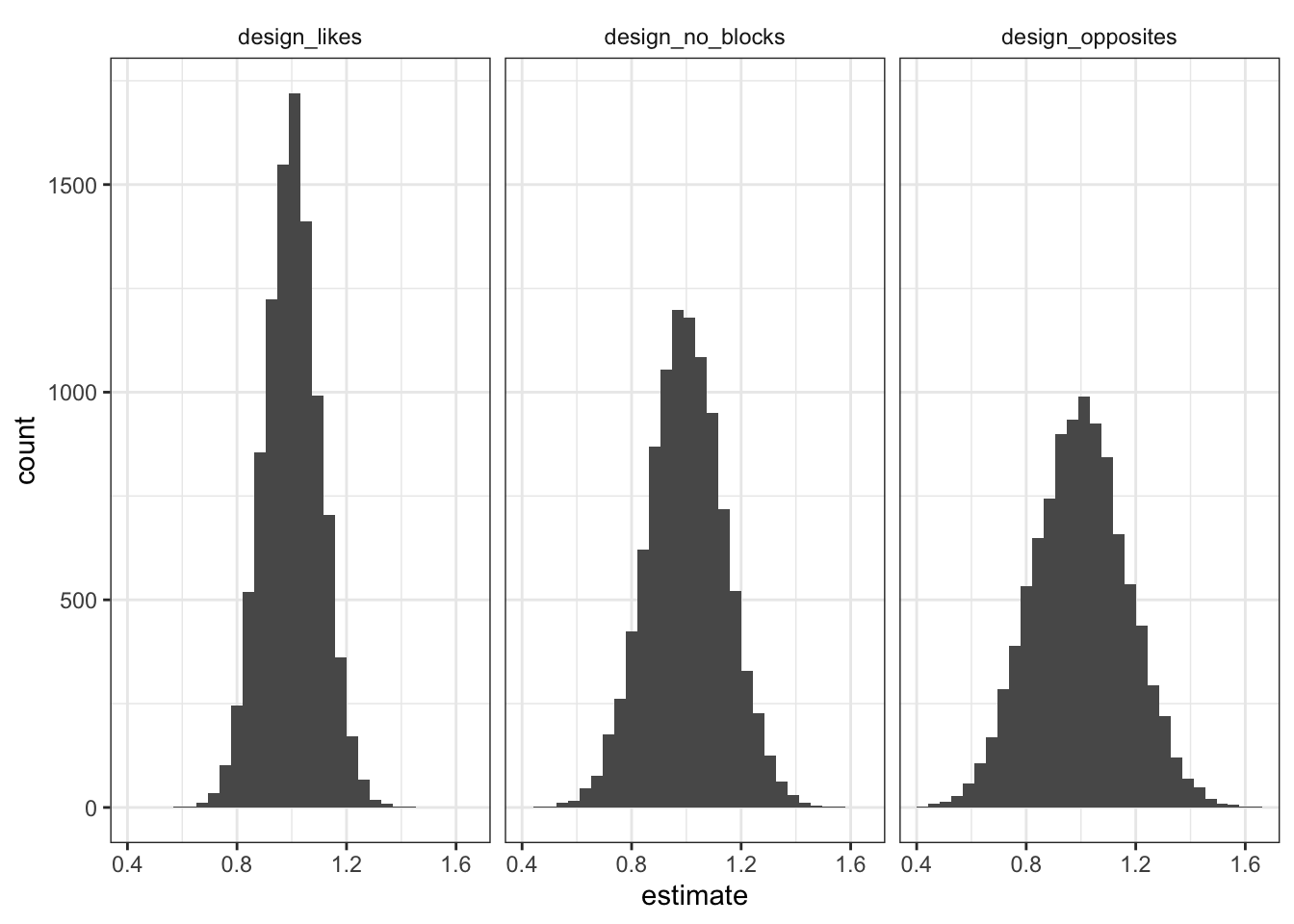

The plots paint a pretty clear picture. All the distributions are centered on 1 (the true average effect), but they vary quite a bit in how dispersed they are—the more dispersed, the more off our answer is likely to be in any given experiment. If we make blocks out of couples that are similar to each other, the sampling distribution is super tight, meaning we have are more likely to be close to the right answer in any given experiment. But if we make blocks out of couples that are very different from each other, we actually do worse than in the no blocking case.

So blocking here will tend to work well if indeed couples are similar on dimensions that are correlated with potential outcomes. But the gains from blocking really depend on the assumption of couples being similar. If in fact “opposites attract,” then blocking on couple can do more harm than good.

We can confirm the graphical intuition by directly calculating the true standard error of each approach.

diagnose_design(design_likes, design_no_blocks, design_opposites,
                diagnosands = declare_diagnosands(sd_estimate = sd(estimate)))

Design	SD Estimate
design_likes	0.102
design_no_blocks	0.143
design_opposites	0.174

So there you have it. It is technically possible that some blocking strategies could make things worse. If you make homogeneous blocks (homogeneous in terms of potential outcomes), blocking helps. But if you make heterogeneous blocks (again in terms of potential outcomes) blocking could hurt.

Size

As discussed in Moore (2012) and Imai, King, and Stuart (2008), “bad blocking” is often only a problem in small samples and can go away if the sample size is sufficiently large.

How small small is will depend on the background model and specifics of the estimand (Imai 2008). For any given model, however, DeclareDesign makes it easy to answer that kind of question. Here we do the same diagnosis as above but with larger designs with \(N\)s of 250 and 2500.

diagnose_design(Like_blocks_250  = redesign(design_likes,     N = 250),
                No_blocks_250    = redesign(design_no_blocks, N = 250),
                Opposites_250    = redesign(design_opposites, N = 250),
                Like_blocks_2500 = redesign(design_likes,     N = 2500),
                No_blocks_2500   = redesign(design_no_blocks, N = 2500),
                Opposites_2500   = redesign(design_opposites, N = 2500),
                diagnosands      = declare_diagnosands(sd_estimate = sd(estimate))

Design	N	SD Estimate
Like_blocks_250	250	0.064
No_blocks_250	250	0.091
Opposites_250	250	0.111
Like_blocks_2500	2500	0.020
No_blocks_2500	2500	0.029
Opposites_2500	2500	0.035

We see here how the loss from bad blocking declines, in absolute terms, with sample size (as does variance in general). In relative terms though we note that we are not seeing clear declines for this design. In the \(N = 100\) case the variance in the sampling distribution with bad blocking is an estimated 47% bigger than the variance with no blocking; for \(N = 250\) it is 50% bigger and for \(N = 2500\) it is 48% bigger.

References

Gerber, Alan S., and Donald P. Green. 2012. Field Experiments: Design, Analysis, and Interpretation. WW Norton.

Imai, Kosuke. 2008. “Variance Identification and Efficiency Analysis in Randomized Experiments Under the Matched-Pair Design.” Statistics in Medicine 27 (24): 4857–73.

Imai, Kosuke, Gary King, and Elizabeth A Stuart. 2008. “Misunderstandings Between Experimentalists and Observationalists about Causal Inference.” Journal of the Royal Statistical Society: Series A (Statistics in Society) 171 (2): 481–502.

Moore, Ryan T. 2012. “Multivariate Continuous Blocking to Improve Political Science Experiments.” Political Analysis 20 (4): 460–79.