design_stub <-

  declare_model(
      N = 195,
      X = rbinom(N, 1, .3) == 1,
      causal_process = sample(c('X_causes_Y', 'X_causes_not_Y', 'Y_regardless', 'not_Y_regardless'),
                              N, replace = TRUE, prob = c(.2, .1, .2, .5)),
      Y = (X & causal_process == "X_causes_Y") |
          (!X & causal_process == "X_causes_not_Y") |
          (causal_process == "Y_regardless"))  +

  declare_sampling(S = strata_rs(strata = (X == 1 & Y == 1),
                                 strata_n = c("FALSE" = 0, "TRUE" = 1))) +

  declare_measurement(
    SIW_observed = rbinom(
      n = N, size = 1, prob = ifelse(test = causal_process == 'X_causes_Y', .75, .25)),
    SMG_observed = rbinom(
      n = N, size = 1, prob = ifelse(test = causal_process == 'X_causes_Y', .3,  .05)),
    label = "Independent Clues") +

declare_inquiry(did_X_cause_Y = causal_process == 'X_causes_Y') Qualitative process-tracing sometimes seeks to answer “cause of effects” claims using within-case data: how probable is the hypothesis that \(X\) did in fact cause \(Y\)? Fairfield and Charman (2017), for example, ask whether the right changed position on tax reform during the 2005 Chilean presidential election (\(Y\)) because of anti-inequality campaigns (\(X\)) by examining whether the case study narrative bears evidence that you would only expect to see if this were true.1 When inferential logics are so clearly articulated, it becomes possible to do design declaration and diagnosis. Here we declare a Bayesian process-tracing design and use it to think through choices about what kinds of within-case information have the greatest probative value.
Say we want to evaluate a case-specific hypothesis, \(H\), regarding whether \(Y\) happened because \(X\) happened. The hypothesis is not that \(X\) is the only cause of \(Y\), but more simply whether \(Y\) would have been different had \(X\) been different. A researcher looks for “clues” or evidence, \(E\), in a case narrative or other qualitative data, which would be more or less surprising to see depending on whether \(H\) is true. Collier (2011) lays out the basic strategy. In a recent paper, Murtas, Dawid, and Musio (2017) show how to justify updating case level inferences from experimental data on moderators and mediators.
Formally declaring and diagnosing such a procedure yields two non-obvious insights:
Straws in the wind can be stronger than smoking guns: Strong but rare clues do not always give you better answers on average than weak but common clues.
The joint distribution of clues can be really important: Many applications of Bayesian process-tracing implicitly assume that clues are generated independently. Yet, when clues are negatively correlated (i.e., they arise through alternative causal pathways), they are jointly much more informative than when they are positively correlated.
Declaring a process-tracing design
There are different approaches to process-tracing. We focus here on “theory testing” rather than exploratory process-tracing and use an approach that draws on the potential outcomes framework (see for example Humphreys and Jacobs (2015)).
We consider a simple example: you choose one country in which there was a civil war (\(Y\)) and natural resources (\(X\)), and look for evidence (\(E\)) that helps you update beliefs about \(Pr(H)\)—the probability that the civil war happened because natural resources were present (H/T Ross (2004)).
Model-Inquiry-Data
If we think of causal relations in counterfactual terms there are just four possible causal relationships between a binary \(X\) and a binary \(Y\):
The presence of natural resources could cause civil war (\(X\) causes \(Y\)).
The presence of natural resources could be the only thing preventing war (\(\neg X\) causes \(Y\)).
Civil war might happen irrespective of whether natural resources are present (\(Y\) irrespective of \(X\)).
Civil war might not happen irrespective of whether natural resources are present (\(\neg Y\) irrespective of \(X\)).
For the simulations, we will imagine we are in a world with 195 countries of which roughly 30% have natural resources (\(X\)) (that’s easy to specify). We will also specify a model in which civil war is governed by causal pathway 1 (\(X\) causes \(Y\)) in roughly 20% of countries, by pathway 2 (\(\neg X\) causes \(Y\)) in only 10% of countries, by pathway 3 (\(Y\) irrespective of \(X\)) in 20% of countries, and by pathway 4 (\(\neg Y\) irrespective of \(X\)) in half of all countries (that’s not so easy to specify and of course is information that is not available at the answer stage).
In addition, we imagine that there is further “process” data that is informative about causal relations. We imagine two types (see Collier (2011) for a discussion of clues of this type):
A straw-in-the-wind clue. A straw-in-the-wind clue is an outcome that is somewhat more likely to be present if the hypothesized causal process is in operation and somewhat less likely if it is not. Let’s say, for example, that \(E_1\) is the national army taking control over natural resources during a civil war. We imagine that that’s likely to happen if the natural resources caused the war: \(Pr(E_1 \mid H) = .75\). But even if the natural resources didn’t cause the war, the national army might still take over natural resources for other reasons, say \(Pr(E_1 \mid \neg H) = .25\).
A smoking gun clue. A smoking gun clue is an outcome that is somewhat likely to be present if the stipulated hypothesis is true, but very unlikely if it is false. Say one of the antagonists was an armed group whose main name, aims, and ideology were centered around the capture and control of natural resources. This information provides a clue which might be really unlikely to arise in general, even if \(H\) is true. But it’s very informative if it is observed, since it’s so unlikely to arise if \(H\) is not true: it’s a “smoking gun.” Let’s say \(Pr(E_2 \mid H) = .3, Pr(E_2 \mid \neg H) = 0.05\).
These clues might themselves be mediators, or moderators, or even arise post treatment, though we do not specify the full causal model that gives rise to them here. Rather, we simply define a step that generates these clue observations independently, conditional on the causal process. This is a strong assumption: the fact that an armed group formed in order to take resources (\(E_2\)) might convince the government to take over the natural resource (\(E_1\)) – or it might dissuade the government! We therefore relax this “Independent Clues” assumption below.
This gives us enough information to put down the stub of a design in which a model generates data with these features, an imaginary researcher samples one case from the \(X=Y=1\) group, and defines the question the researcher wants to ask about this case. Notice here the inquiry takes place after the sampling because we care about what happens in the specific case we chose.
So far, a dataset from this design stub might look like this:
draw_data(design_stub) %>% kable(digits = 2, align = "c")| ID | X | causal_process | Y | S | SIW_observed | SMG_observed |
|---|---|---|---|---|---|---|
| 055 | TRUE | X_causes_Y | TRUE | 1 | 1 | 0 |
Answer strategy
We now turn to the answer strategy. For this, we’ll assume that at the analysis stage researchers use Bayes’ rule to figure out \(Pr(H \mid E)\): the posterior probability that \(X\) caused \(Y\) in the case we chose, given the clue evidence we found. We make a function that calculates the posterior using Bayes’ rule:
\[Pr(H \mid E) = \frac{Pr(H) Pr(E|H)}{Pr(H)Pr(E\mid H) + Pr(\neg H)Pr(E\mid\neg H)}\]
calculate_posterior <- function(data, p_H, p_clue_found_H, p_clue_found_not_H, test, label) {
  clue_found <- data[, test]
  p_E_H <- ifelse(clue_found, p_clue_found_H, 1 - p_clue_found_H)
  p_E_not_H <- ifelse(clue_found, p_clue_found_not_H, 1 - p_clue_found_not_H)
  data.frame(posterior_H = p_E_H * p_H / (p_E_H * p_H + p_E_not_H * (1 - p_H)), clue_found = clue_found)}
Bayes’ rule makes use of the probability of observing \(E\) if \(H\) is true and the probability of observing \(E\) if \(H\) is not true. The more different these probabilities are the more you learn from new data.
We also need to specify the imaginary researcher’s prior belief that \(H\) is true. The imaginary researcher knows that only two processes, 1 and 3 from above, could have generated the data \(X = Y = 1\). Thus, they might specify a “flat” prior: \(Pr(H) = .5\) (though they might have more informed beliefs from background knowledge).
We use the calculate_posterior() function we made above to declare two different answer strategies: one predicated on the straw-in-the-wind, and the other on the smoking gun.
design <-

  design_stub +

  declare_estimator(
    test               = "SIW_observed",
    p_H                = .5,
    p_clue_found_H     = .75,
    p_clue_found_not_H = .25,
    label              = "Straw in Wind",
    estimand           = "did_X_cause_Y",
    handler            = label_estimator(calculate_posterior)) +

  declare_estimator(
    test               = "SMG_observed",
    p_H                = .5,
    p_clue_found_H     = .30,
    p_clue_found_not_H = .05,
    label              = "Smoking gun",
    estimand           = "did_X_cause_Y",
    handler            = label_estimator(calculate_posterior))
Diagnosis
With this declaration, we can use simulate_design(design) to simulate the design many times, and then see how the strategies perform on average.
Below we plot the distribution of inferences, \(Pr(H|E)\), given strategies and true causal processes. The dotted lines show the true values of \(Pr(H)\). The left column represents guesses when conditioning on the straw-in-the-wind, whereas the right column represents guesses when conditioning on the smoking gun. In both cases, the results are “unbiased” (yes we can assess bias from diagnosis even for a Bayesian design)—because it so happened here that the distribution of causal pathways specified for the background model and the true probabilities of the clues matched the those used in the researcher’s answer strategy.
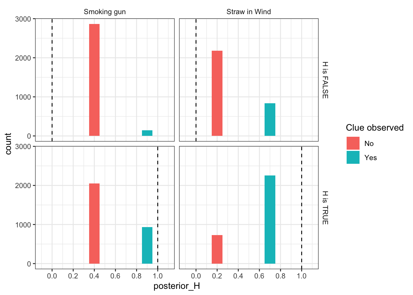
As expected, the smoking gun can be highly probative: the bottom right panel shows that we sometimes get the answer exactly right (i.e., in those cases when \(H\) is true and we observe a smoking gun). Note, however, that this is pretty rare: most of the time we guess \(Pr(H\mid E_2) =\) 0.25, which is quite far from the true values of 0 and 1. We sometimes, but very rarely, get a false smoking gun. The smoking gun distribution is one that is centered close to the prior but sometimes makes big, and usually correct, inferential leaps.
By contrast, the left column shows that the straw-in-the-wind strategy gets pretty close pretty often. Whenever it is observed, the researcher guesses \(Pr(H\mid E_1) =\) 0.86, and when it is not they guess \(Pr(H\mid E_1) =\) 0.42. This means they sometimes make mistakes – because they observe \(E_1\) even when \(H\) is false, and vice versa. But it happens rarely enough that they tend to move in the right direction most of the time.
The net result is that, in this case, the straw-in-the-wind test has lower root mean squared error (RMSE): 0.47 vs. the smoking gun’s 0.44. It’s less wrong more often. In general, however, which type of clue provides better inferences depends on the particular probabilities assumed.
Using more than one clue
In practice, researchers seldom pre-commit to updating from a single piece of evidence, but search for multiple clues and update about their cause of effects hypotheses jointly. As mentioned above, however, doing so in fact requires that we specify the joint distribution of the clues.
In the code appendix below, we create a function (joint_prob()) for specifying the joint distribution of the clues, given their marginal probabilities and the correlation between them (rho). We also replace the “Independent Clues” step with a “Correlated Clues” step, in which clues arise according to this joint distribution. This enables us to add a strategy in which we update in light of both clues simultaneously.
We skip that code here, and simply show how the RMSE changes as a function of rho for the three different strategies.
`summarise()` has grouped output by 'rho_H'. You can override using the
`.groups` argument.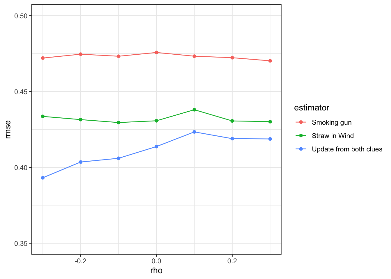
As expected, using more information (both of the clues) gets you much better answers on average. However, notice that the gains from a joint approach are much greater when the clues are negatively correlated than when they are positively correlated.
This feature arises because the pieces of evidence carry less independent information when they are positively correlated. To see this, suppose they were perfectly correlated, so that observing one clue guarantees that you would observe the other. In this case, there is no additional information gleaned from the observation of one clue once the other has been observed: they are effectively equivalent tests. So, one implication is that process-tracers may do better by looking for clues that are negatively correlated. What might this look like in practice?
Negatively correlated clues might arise if they result from processes that substitute for each other. For example, if the national army is less likely to take control of the natural resources precisely when an armed group has declared that it will fight for them. Positively correlated clues might arise if they result from common processes. For example, if the national army takes control over natural resources precisely because this counters the stated strategic objectives of the armed group.
Takeaways
We see four main takeaways here:
The frequency of clues matters: against much of the advice in the process-tracing literature,2 a researcher who had to choose one clue to make an inference would do better to choose a straw-in-the-wind than a smoking gun.
The joint distribution of clues matters: very often we would expect clues to arise through interrelated causal processes. Researchers can in fact make more powerful inferences if they can defend the assumption that clues are negatively correlated.
Declaring and diagnosing designs forces you to think them through in a way that can make non-obvious features and assumptions obvious. At a minimum, formalizing your design in this manner can highlight what kinds of beliefs are necessary to justify inferences.
With that said, we also see here a lesson on the limits of declaration. Even with just two clues, declaring a process-tracing inferential strategy makes serious demands on researcher knowledge. In particular, the ability to make claims about the joint distribution of clues under alternative causal hypotheses. In principle, it is possible to base such beliefs on external data (see Murtas, Dawid, and Musio (2017)) but doing so is hard and the challenges rise exponentially as more and more complex clues are considered. The declaration strategy works best, perhaps, for major claims resulting from key evidence. It seems unlikely to be able to capture inferences made from all the complex evidence used by process tracers.
Code appendix
# Calculate bivariate probabilities given correlation
joint_prob <- function(p1, p2, rho) {
  r <- rho * (p1 * p2 * (1 - p1) * (1 - p2)) ^ .5
  c(`00` = (1 - p1) * (1 - p2) + r,
    `01` = p2 * (1 - p1) - r,
    `10` = p1 * (1 - p2) - r,
    `11` = p1 * p2 + r)}

rho_H <- 0
rho_not_H <- 0

calculate_posterior_joint <- function(data, p_H, p_clue_1_found_H, p_clue_1_found_not_H, p_clue_2_found_H, p_clue_2_found_not_H, rho_H, rho_not_H, test){
  clue_found <- data[, test]
  p_E_H <- joint_prob(p1 = p_clue_1_found_H, p2 = p_clue_2_found_H, rho = rho_H)[clue_found]
  p_E_not_H <- joint_prob(p1 = p_clue_1_found_not_H, p2 = p_clue_2_found_not_H, rho = rho_not_H)[clue_found]
  data.frame(posterior_H = p_E_H * p_H / (p_E_H * p_H + p_E_not_H * (1 - p_H)), clue_found = clue_found)
}

corr_design <- replace_step(
  design = design,
  step = "Independent Clues",
  new_step =  declare_step(
    SIW_SMG = sample(c("00", "01", "10", "11"),1,
                     prob = {
                       if(causal_process == "X_causes_Y")
                         joint_prob(.75, .30, rho_H)
                       else
                         joint_prob(.25,  .05, rho_not_H)
                     }),
  SIW_observed = SIW_SMG == "10" | SIW_SMG == "11",
  SMG_observed = SIW_SMG == "01" | SIW_SMG == "11",
  handler = fabricate,
  label = "Correlated Clues"))

corr_design <- corr_design +
  declare_estimator(
    test                 = "SIW_SMG",
    p_H                  = .5,
    p_clue_1_found_H     = .75,
    p_clue_1_found_not_H = .25,
    p_clue_2_found_H     = .30,
    p_clue_2_found_not_H = .05,
    rho_H                = rho_H,
    rho_not_H            = rho_not_H,
    label                = "Update from both clues",
    estimand             = "did_X_cause_Y",
    handler              = label_estimator(calculate_posterior_joint))
References
Collier, David. 2011. “Understanding Process Tracing.” PS: Political Science & Politics 44 (4): 823–30.
Fairfield, Tasha, and Andrew E. Charman. 2017. “Explicit Bayesian Analysis for Process Tracing: Guidelines, Opportunities, and Caveats.” Political Analysis 25 (3): 363–80.
Humphreys, Macartan, and Alan M Jacobs. 2015. “Mixing Methods: A Bayesian Approach.” American Political Science Review 109 (4): 653–73.
Murtas, Rossella, Alexander Philip Dawid, and Monica Musio. 2017. “New Bounds for the Probability of Causation in Mediation Analysis.” arXiv Preprint arXiv:1706.04857.
Ross, Michael L. 2004. “How Do Natural Resources Influence Civil War? Evidence from Thirteen Cases.” International Organization 58 (1): 35–67.
Footnotes
For example: “the former President [said] that the tax subsidy ‘never would have been eliminated if I had not taken [the opposition candidate] at his word’ when the latter publicly professed concern over inequality.”↩︎
E.g. Collier (2011): of the four process-tracing tests, straws-in-the-wind are ``the weakest and place the least demand on the researcher’s knowledge and assumptions.’’ (826)↩︎