Most power calculators take a small number of inputs: sample size, effect size, and variance. Some also allow for number of blocks or cluster size as well as the overall sample size. All of these inputs relate to your data strategy. Unless you can control the effect size and the noise, you are left with sample size and data structure (blocks and clusters) as the only levers to play with to try to improve your power.

In fact, though, power depends on your answer strategy and not just your data strategy and so you might do better putting resources into improving what you do with your data rather than the amount of data you have.

Power from the answer strategy

Random assignment generally means that you do not have to include control variables in an analysis in order to achieve unbiasedness. But including controls can improve precision and increase power. If you are trying to improve your power but adding observations is expensive, perhaps you should first explore whether you can improve power by adjusting the estimation approach.

Here is an illustration of a two-arm trial with 40 units in which 20 units are assigned to treatment, blocking on a binary pre-treatment covariate \(W\). We’ll let the treatment effects vary according to \(W\), but the true average treatment effect (our estimand in this case) is equal to 1.

N = 40

# Model
model <- declare_model(N, W = rep(0:1, N / 2), u = rnorm(N), potential_outcomes(Y ~ 2 * Z * W + u))  

# Inquiry
inquiry     <- declare_inquiry(ate = 1)  

# Data strategy
assignment   <- declare_assignment(Z = block_ra(blocks = W))
measurement  <- declare_measurement(Y = reveal_outcomes(Y ~ Z))

# Answer strategy
estimator  <- declare_estimator(Y ~ Z, estimand = "ate", label = "Simple D-I-M")

# Declare the design
design <- model + inquiry + assignment + measurement + estimator

Under this data generating process, the treatment interacts quite strongly with \(W\). The average effect of treatment is 1, but the conditional average treatment effects are 0 and 2 for the two levels of \(W\). The difference-in-means analysis strategy for this design is equivalent to an OLS regression of the outcome on the treatment with no control variables included. Because of random assignment, this procedure is of course unbiased, but it leaves money on the table in the sense that we could achieve higher statistical power if we included information about \(W\) in some way. Here is the power of the difference-in-means answer strategy:

diagnose_design(design)

Inquiry	RMSE	Power	Coverage	Mean Estimate	SD Estimate	Mean Se	Type S Rate	Mean Estimand	N Sims
ate	0.32	0.75	0.98	1.00	0.32	0.39	0.00	1.00	10000

So power is good though short of conventional standards. Based on this diagnosis the probability of getting a statistically significant result is only 0.75 even though the true effect is reasonably large.

Let’s consider two additional estimation strategies. The first controls for the pre-treatment covariate \(W\) in an OLS regression of the outcome on treatment plus the covariate. This strategy is the standard approach to the inclusion of covariates in experimental analysis. An alternative is the “Lin estimator,” so named by us because of the lovely description of this approach given in Lin (2013). This estimator interacts treatment with the de-meaned covariates. The lm_lin() function in the estimatr package implements the Lin estimator for easy use.

Here is the expanded design and the diagnosis:

new_design <- design +
              declare_estimator(Y ~ Z + W,  model = lm_robust,
                                inquiry = "ate", label = "OLS: Control for W") +
              declare_estimator(Y ~ Z, covariates = ~ W, model = lm_lin,
                                inquiry = "ate", label = "Lin: Control + Interaction")

Estimator	RMSE	Power	Coverage	Mean Estimate	SD Estimate	Mean Se	Mean Estimand	N Sims
Lin: Control + Interaction	0.32	0.87	0.95	1.00	0.32	0.31	1.00	10000
OLS: Control for W	0.32	0.81	0.97	1.00	0.32	0.35	1.00	10000
Simple D-I-M	0.32	0.74	0.99	1.00	0.32	0.39	1.00	10000

We see here a clear ranking of the three estimation strategies in terms of power. You will notice that the coverage also varies across designs: the simple difference in means approach is actually overly conservative in part because it does not take account of the blocked randomization. The OLS model that in some sense “controls for blocks” does better, but is still above the nominal coverage of 95%. In this case, the coverage of the Lin model is excellent.

Tradeoffs

To figure out how these gains in power from switching up estimation strategies compare with gains from increasing \(N\) we declare a sequence of designs, differing only in values for \(N\). We do that in two steps:

designs   <- redesign(new_design, N = seq(30, 80, 10))
diagnoses <- diagnose_design(designs)

The diagnoses object now contains full diagnoses for a whole sequence of designs that assume different \(N\)s and that each contain multiple estimation strategies. Here is a graph of the output showing trade-offs between design size and estimation strategy.

diagnoses$diagnosands_df %>%
  ggplot(aes(N, power)) +
  geom_line(aes(color = estimator))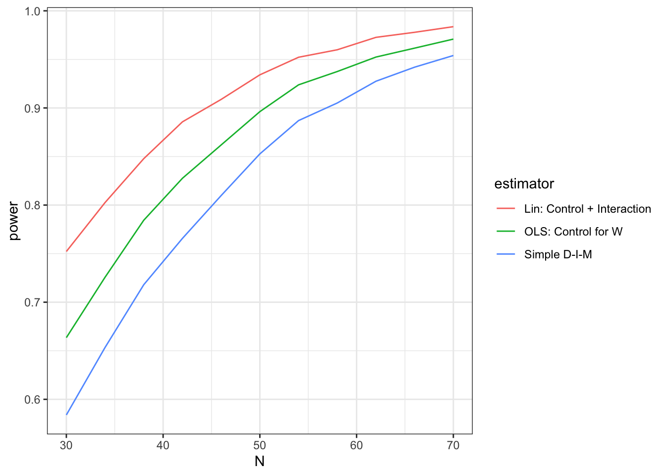

We see here that if you had 45 units and wanted to use simple differences in means your power would be around 80%. You could up your power to just over 90% by increasing the size of the experiment to about 60 units. Or, conditional on speculations about the heterogeneous effects of treatment, you could do the same thing by staying at 45 but switching over to the Lin estimator.

A puzzle

Sometimes researchers coarsen control variables, for example turning a 10 point democracy scale into a binary variable, because they believe the finer scale is noisier. Can you declare a design to assess whether dichotomizing an outcome variable increases or decreases power?

References

Lin, Winston. 2013. “Agnostic Notes on Regression Adjustments to Experimental Data: Reexamining Freedman’s Critique.” The Annals of Applied Statistics 7 (1): 295–318.