You’re partnering with an education nonprofit and you are planning on running a randomized control trial in 80 classrooms spread across 20 community schools. The request is in: please send us a spreadsheet with random assignments. The assignment’s gotta be blocked by school, it’s gotta be reproducible, and it’s gotta be tonight. The good news is that you can do all this in a couple of lines of code. We show how using some DeclareDesign tools and then walk through handling of more complex cases.

You can do it!

We’ll show first how you do it and then talk through some of the principles, wrinkles, and checks you might do. Here’s the code:

library(DeclareDesign)

set.seed(20181204)

here_you_go <- fabricate(school = add_level(N = 20),
                         class  = add_level(N = 4, treatment = block_ra(blocks = school)))

The spreadsheet looks like this:

school	class	treatment
01	01	0
01	02	1
01	03	0
01	04	1
02	05	0
02	06	1
02	07	0
02	08	1
03	09	1
03	10	1
03	11	0
03	12	0
04	13	0
04	14	1
04	15	1
04	16	0
05	17	0
05	18	1
05	19	1
05	20	0
06	21	1
06	22	0
06	23	0
06	24	1
07	25	0
07	26	1
07	27	1
07	28	0
08	29	0
08	30	0
08	31	1
08	32	1
09	33	0
09	34	1
09	35	1
09	36	0
10	37	0
10	38	0
10	39	1
10	40	1
11	41	1
11	42	0
11	43	0
11	44	1
12	45	0
12	46	1
12	47	1
12	48	0
13	49	0
13	50	1
13	51	1
13	52	0
14	53	0
14	54	1
14	55	0
14	56	1
15	57	0
15	58	1
15	59	1
15	60	0
16	61	0
16	62	1
16	63	0
16	64	1
17	65	0
17	66	0
17	67	1
17	68	1
18	69	0
18	70	1
18	71	0
18	72	1
19	73	1
19	74	0
19	75	1
19	76	0
20	77	0
20	78	1
20	79	1
20	80	0

It has 20 schools with 4 classes in each and in each school exactly 2 classes are randomly assigned to treatment. The class variable provides a unique identifier for the experimental units.

The basic work here is done in a single line of code using fabricate from the fabricatr package and block_ra from the randomizr package. The fabricatr package helped us make a multilevel dataset (using add_level) and the randomizr package lets us specify what we want to use as blocks for a blocked random assignment.

You can then save this as a spreadsheet and send off:

write.csv(here_you_go, file = "our_assignment_final_revised_final_version_3_latest.csv")

We’re done.

Some principles and a better workflow

We got the job done. How well did the approach do in terms of satisfying various randomization desiderata?

We want random assignment to be transparent in the sense that the process by which units were assigned to treatment conditions is fully understandable to interested parties. The code here provides much of the needed transparency. One point of slippage perhaps here is that the there is no specification for how the units here map into the actual units in the field. There should be no ambiguity as to which classroom we are talking about when we talk about classroom 5 in school 2. If this mapping can be determined later then the randomization can come undone.
We want the random assignment to be reproducible in the sense that a person using the same software could generate the same random assignment. This is typically assured by setting a random number seed (set.seed(20181204)). If you give the computer a “seed” before randomizing you will get the same “random” result every time. Setting seeds produces a small risk to transparency since in principle one could select a seed to get a result you like. One approach used here is to use a rule for seed setting – such as setting the seed as the date of the randomization. Another is to publicly post a single seed that you or your lab will use for all projects.
We want to be able to verify properties of the random assignment procedure, not just of a particular assignment. For that, we need to be able to generate many thousands of possible random assignments. It helps immensely if the random assignment procedure is itself a function that can be called repeatedly, rather than a script or a point-and-click workflow. We have not done that here so will walk through that below.

Rather than writing code that produces an assignment and dataframe directly it can be useful to write down a procedure for generating data and assignment. DeclareDesign functions are good for this since these are mostly functions that make functions.

make_data  <- declare_model(school = add_level(N = 20),
                            class  = add_level(N = 4))
assignment <- declare_assignment(Z = block_ra(blocks = class))

With these functions (make_data() and assignment() are functions!) written up, you have both the data structure and the assignment strategy declared. There are many ways now to run these one after another to generate a dataset with assignments. Some examples:

our_assignment <- assignment(make_data())     # base R approach 

our_assignment <- make_data() %>% assignment  # dplyr approach

The base R approach and the dplyr approach both run the first function and then apply the second function to the result.

We advocate a design declaration approach that first concatenates the two steps into a design and then draws data using the design.

design         <- make_data + assignment
our_assignment <- draw_data(design)           # DeclareDesign approach

school	class	Z
01	01	1
01	02	1
01	03	0
01	04	0
02	05	1
02	06	0
02	07	1
02	08	1
03	09	1
03	10	1
03	11	0
03	12	0
04	13	1
04	14	0
04	15	1
04	16	0
05	17	0
05	18	0
05	19	0
05	20	0
06	21	0
06	22	0
06	23	1
06	24	1
07	25	1
07	26	0
07	27	1
07	28	0
08	29	0
08	30	1
08	31	1
08	32	0
09	33	1
09	34	0
09	35	0
09	36	0
10	37	1
10	38	0
10	39	1
10	40	1
11	41	1
11	42	0
11	43	0
11	44	0
12	45	1
12	46	0
12	47	0
12	48	0
13	49	1
13	50	1
13	51	1
13	52	0
14	53	0
14	54	1
14	55	0
14	56	1
15	57	1
15	58	0
15	59	0
15	60	1
16	61	1
16	62	0
16	63	0
16	64	0
17	65	0
17	66	0
17	67	0
17	68	0
18	69	0
18	70	1
18	71	1
18	72	0
19	73	1
19	74	1
19	75	1
19	76	1
20	77	0
20	78	0
20	79	1
20	80	0

A nice feature of the last approach is that not only can you conduct an actual random assignment from the design but you also obtain the probability that each unit is in the condition that it is in. This probability happens to be constant in this example, but it doesn’t need to be. If probabilities vary by unit, a standard approach is to weight each unit by the inverse of the probability of being in the condition that it is in.

We will use this last approach going forward as we look at more bells and whistles.

Four bells and whistles

Incorporate known data into a dataframe before randomization

In general the world is not quite as neat as in the example above. Say in fact our data came in like this (of course it would be easier if you were sent a nice dataset but you cannot always count on that):

Just got the numbers: School 1 has 6 classes, school 2 has 8, schools 4 and 8 have 3 classes, schools 5 and 9 have 5, school 6 has 2, school 10 has 7. Remember we need this yesterday.

We want to incorporate this information in the data fabrication step. The add_level functionality in the fabricate function is key here for respecting the multilevel nature of the dataset.

make_data <- declare_model(
  school = add_level(N = 10),
  class  = add_level(N = c(6, 8, 4, 3, 5, 2, 4, 3, 5, 7)))

This new function would generate a data set that reflects the number of classes in each school.

Make better blocks from richer data

Say that you had even richer data about the sampling frame. Then you could use this to do even better assignments. Say this is what you get from your partner:

We just got information on the class sizes. Here it is: School 1: 20, 25, 23, 30, 12, 15; School 2: 40, 42, 53, 67, 35, 22, 18, 18; School 3: 34, 37, 28, 30; School 4: 18, 24, 20; School 5: 10, 24, 13, 26, 18; School 6: 20, 25; School 7: 28, 34, 19, 24; School 8: 32, 25, 31; School 9: 23, 20, 33, 22, 35; School 10: 20, 31, 34, 35, 18, 23, 22

We want to incorporate this information in the data fabrication step.

make_data <- declare_model(
    school = add_level(N = 10),
    class = add_level(N = c(6, 8, 4, 3, 5, 2, 4, 3, 5, 7),
                size = c(
                  20, 25, 23, 30, 12, 15,         # students in each classroom of school 1
                  40, 42, 53, 67, 35, 22, 18, 18, # students in each classroom of school 2
                  34, 37, 28, 30,                 # etc...
                  18, 24, 20,
                  10, 24, 13, 26, 18,
                  20, 25,
                  28, 34, 19, 24,
                  32, 25, 31,
                  23, 20, 33, 22, 35,
                  20, 31, 34, 35, 18, 23, 22
                )))

This new data on class sizes might be very useful.

If the NGO wants to examine individual level outcomes but is using a classroom-level intervention, then this design is using “clustered” random assignment (students clustered into classrooms). As noted in Imai et al. (2009), however, if clusters are of uneven sizes, standard estimation approaches can be biased, even though it’s a randomized experiment. They propose blocking on cluster size in order to address this problem. We’ll use blockTools (by Ryan T. Moore and Keith Schnakenberg) to block on both school and classroom size within schools.

The block function within blockTools forms blocks as a function of size by pairing similarly-sized classrooms (blocks of size 2 is the default for the block function, though this can be changed). By telling the function that classes are grouped within schools, we can ensure that blockTools will pair classrooms within the same school. We turn this functionality into a design step like this:

# A step to generate blocks
block_function <- function(data) {
    out <- block(data, id.vars = "class", groups = "school", block.vars = "size")
    mutate(data, block_id = createBlockIDs(out, data, id.var = "class"))}

make_blocks <- declare_step(handler =  block_function)

Let’s make a design that includes this step and now uses block_id instead of class for blocking:

design <- make_data + make_blocks + declare_assignment(Z = block_ra(blocks = block_id))

When we draw data we now get the block variables and the assignment probabilities included. One out of two units is assigned to each block of two and singleton blocks are assigned independently with 0.5 probability to treatment.

our_df <- draw_data(design)

school	class	size	block_id	Z
01	01	20	3	0
01	02	25	1	1
01	03	23	1	0
01	04	30	3	1
01	05	12	2	0
01	06	15	2	1
02	07	40	5	0
02	08	42	5	1
02	09	53	7	0
02	10	67	7	1
02	11	35	6	1
02	12	22	6	0
02	13	18	4	0
02	14	18	4	1
03	15	34	9	0
03	16	37	9	1
03	17	28	8	1
03	18	30	8	0
04	19	18	10	1
04	20	24	11	1
04	21	20	10	0
05	22	10	13	0
05	23	24	12	0
05	24	13	13	1
05	25	26	12	1
05	26	18	14	1
06	27	20	15	0
06	28	25	15	1
07	29	28	16	1
07	30	34	17	1
07	31	19	17	0
07	32	24	16	0
08	33	32	18	0
08	34	25	19	0
08	35	31	18	1
09	36	23	20	0
09	37	20	22	1
09	38	33	21	0
09	39	22	20	1
09	40	35	21	1
10	41	20	25	0
10	42	31	26	1
10	43	34	23	1
10	44	35	23	0
10	45	18	25	1
10	46	23	24	1
10	47	22	24	0

The graph below shows that indeed, the blocking formed pairs of classrooms within each school that are similar to one another and correctly left some classrooms in a block by themselves when there was an odd number of classrooms in a school.

our_df %>%
  ggplot(aes(size, block_id, color = as.factor(Z))) +
  geom_point() +
  facet_wrap(~school, scales = "free_y", ncol = 5)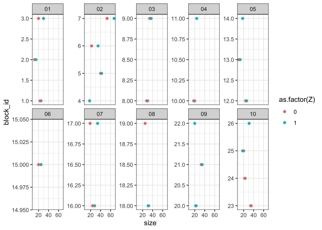

Replicate yourself

If you set up your assignments as functions like this then it is easy to implement the assignment multiple times:

many_assignments <- replicate(1000, draw_data(design))

It’s useful to preserve a collection of assignments like this. One advantage is that it lets you see directly what the real assignment probabilities are—not just the intended assignment probabilities. This is especially useful in complex randomizations where different units might get assigned to treatment with quite different probabilities depending on their characteristics (for instance a procedure that rejects assignment profiles because of concerns with imbalance). Calculating the actual probabilities lets you figure out if you have set things up correctly and in some cases can even be useful for correcting things at the analysis stage if you have not!¹ In addition the collection of assignments stored in many_assignment are exactly the assignments you should use for some randomization inference tests.

Save the output to an excel spreadsheet

Your partners mightn’t love csv spreadsheets. But you can easily save to other formats.

Many people love Microsoft Excel. Using the writexl package (by Jeroen Ooms) will make them happy:

library(writexl)

set_seed(20181204)

our_df <- draw_data(design)

write_xlsx(our_df, path = "students_with_random_assignment.xlsx")

Summary

Sometimes you need to make data from bits of information. fabricatr can help with that.
Sometimes you need to make blocks from multiple pieces of information. blockTools can help with that.
Sometimes you need to conduct a random assignment (and make sure it’s reproducible). The functions in randomizr can help with that.
Sometimes you need to share data with people who use Excel. writexl can help with that!
Think of all this together as a part of a design declaration and you get a guarantee that all the bits do fit together in a transparent and replicable way, plus you are half way to a full declaration.

References.

Imai, Kosuke, Gary King, Clayton Nall, et al. 2009. “The Essential Role of Pair Matching in Cluster-Randomized Experiments, with Application to the Mexican Universal Health Insurance Evaluation.” Statistical Science 24 (1): 29–53.

Footnotes

Some tools in the randomizr package make it even easier to obtain matrices of permutations and to learn about properties of your assignments. Using the randomizr package you can declare a randomization like this ra_declaration <- declare_ra(blocks = class) and then get a print out of features of the assignments using summary(ra_declaration) and a whole matrix of assignments like this perm_mat <- obtain_permutation_matrix(ra_declaration)↩︎