In many experiments, different groups of units get assigned to treatment with different probabilities. This can give rise to misleading results unless you properly take account of possible differences between the groups. How best to do this? The go-to approach is to “control” for groups by introducing “fixed-effects” in a regression set-up. The bad news is that this procedure is prone to bias. The good news is that there’s an even simpler and more intuitive approach that gets it right: estimate the difference-in-means within each group, then average over these group-level estimates weighting according to the size of the group. We’ll use design declaration to show the problem and to compare the performance of this and an array of other proposed solutions.

The trouble

For intuition, imagine a design that has experimental blocks (these might correspond to geographic regions or gender groups, for example). In block A, we treat 1/3 of the units and in block B, we treat 1/2. We are interested in an outcome \(Y\), income, for example. We worry though that if income is higher in group B than group A that we will have introduced a correlation between treatment and outcomes even if there is no causal effect of treatment on income. We want to avoid that kind of false inference.

A good way to think about the problem is to recognize that the overall average treatment effect can be thought of as an average of the average treatment effects in each block. Luckily, figuring out the average effect within a block is not hard. We can think of each block as its own mini-experiment. Within each block all units are treated with the same probability and so difference-in-means estimation within a block works fine to get at the average effect for units in that block. In order to get an overall ATE estimate, we then just have to average the block level estimates together. So if we weight the within-group effects together by \(n_j\) (the size of block \(j\)), we have an unbiased estimator of the ATE.

Simple enough.

But in practice researchers often try to do this calculation using “block fixed effects,” i.e., include a set of block dummies in a regression of the outcome on treatment assignment. The problem though is that while fixed-effects regression does average across within-block average effects, it does so using the wrong weighting scheme. The regression weights are \(p_j(1-p_j)n_j\), where share \(p_j\) of \(n_j\) units are treated within block \(j\). Fixed-effects OLS essentially puts more weight on the blocks with the greatest variance in the treatment variable.¹

Let’s demonstrate the issue using DeclareDesign and then move on to examining different solutions.

First, we declare a design that has three equally-sized blocks, with block-specific effects (tau) and assignment probabilities (prob). We will use three answer strategies: simple regression of the outcome on the treatment indicator (Naive Pooled), a regression of the outcome on the treatment indicator and block fixed effects (Least Squares Dummy Variables), and a sample-weighted average of the within-block difference-in-means (Blocked DIM). We will use a design where the noise is quite small relative to the error to clarify that that the problem is not about precision.

Here’s the design declaration:

# Model ------------------------------------------------------------------------
U <- declare_model(block = add_level(N = 3,
                                     prob = c(.5, .7, .9),
                                     tau = c(4, 2, 0)),
                   indiv = add_level(N = 100, e = rnorm(N), 
                                     Y_Z_0 = e,
                                     Y_Z_1 = e + tau))
# Inquiry ----------------------------------------------------------------------
Q <- declare_inquiry(ATE = mean(Y_Z_1 - Y_Z_0))

# Data Strategy ----------------------------------------------------------------
Z <- declare_assignment(Z = block_ra(blocks = block, block_prob = c(.5, .7, .9)),
                        Z_cond_prob = obtain_condition_probabilities(assignment = Z, blocks = block, block_prob = c(.5, .7, .9)))
R <- declare_measurement(Y = reveal_outcomes(Y ~ Z))

# Answer Strategy --------------------------------------------------------------
A0 <- declare_estimator(Y ~ Z, inquiry = Q,  
                        model =  lm_robust, label = "A0: Naive (Pooled)")
A1 <- declare_estimator(Y ~ Z + block, inquiry = Q,  
                        model =  lm_robust, label = "A1: LSDV")
A2 <- declare_estimator(Y ~ Z, blocks = block, inquiry = Q,  
                        model =  difference_in_means, label = "A2: Blocked DIM")

# Design -----------------------------------------------------------------------
design <- U + Z + Q + R + A0 + A1 + A2

Diagnosis of this design lets us see how these different strategies perform:

diagnose_design(design, sims = sims)

Estimator	Bias	RMSE	Power	Coverage	Mean Estimate	SD Estimate	Mean Se	Mean Estimand	N Sims
A0: Naive (Pooled)	-0.38	0.40	1.00	0.33	1.62	0.13	0.17	2.00	10000
A1: LSDV	0.58	0.59	1.00	0.08	2.58	0.13	0.20	2.00	10000
A2: Blocked DIM	-0.00	0.15	1.00	0.95	2.00	0.15	0.15	2.00	10000

The difference-in-means approach does a good job of estimating the true average treatment effect in the sample. The two other approaches get it terribly wrong.

It’s easy enough to see why the pooled estimator gets things wrong. In this design, the blocks with bigger treatment probabilities also have smaller outcomes in the treatment condition. This creates a negative relation between treatment and outcomes that pulls down the estimate of effects.

But, oddly, the fixed effects estimators is not just biased, it is biased in the opposite direction of the bias of the pooled estimator. Why is that?

Why do fixed effects get it wrong?

We can use the design to drill down and see where this bias from the fixed effects estimator is coming from. We will use the design to generate simulated data and to run our estimators on that single draw.²

one_draw <- draw_data(design)
A1(one_draw)
A2(one_draw)

Warning in fn(data, ~(Y ~ Z + block), model = ~lm_robust): The argument 'model
= ' is deprecated. Please use '.method = ' instead.

Warning in fn(data, ~(Y ~ Z), blocks = ~block, model = ~difference_in_means):
The argument 'model = ' is deprecated. Please use '.method = ' instead.

estimator	estimate
A1: LSDV	2.483
A2: Blocked DIM	1.914

With this simulated data we can calculate the within block effects and the block weights “by hand” to see how the differences-in-means approach and the fixed effects approach do things differently. For this we use dplyr functionality which makes it easy to operate within multiple blocks in parallel.

within_block <-
  one_draw %>%
  group_by(block) %>%
  summarise(block_ATE     = mean(Y_Z_1 - Y_Z_0),
            block_ATE_est = mean(Y[Z == 1]) - mean(Y[Z == 0]),
            n_j = n(),
            p_j = mean(Z),
            sample_weight = n_j,
            fe_weight     = p_j * (1 - p_j) * n_j) %>%
  # divide by the sum of the weights
  mutate(sample_weight = sample_weight/sum(sample_weight),
         fe_weight = fe_weight/sum(fe_weight))

block	block_ATE	block_ATE_est	n_j	p_j	sample_weight	fe_weight
1	4	4.06	100	0.5	0.33	0.45
2	2	1.66	100	0.7	0.33	0.38
3	0	0.02	100	0.9	0.33	0.16

This table helps explain the bias: one-third of the sample has an ATE estimate of 4.06, one-third has an ATE estimate of 1.66, and one-third an estimate of 0.02. Yet, the fixed effects estimator attributes those block-level estimated effects weights of 45%, 38%, and 16%, respectively: it exaggerates the true average effect by overweighting blocks with large effects and underweighting blocks with small effects.

To finish the example, see that we can recover the fixed effects and block DIM estimates from the within block estimates, just by choosing a different weighting strategy.

within_block %>%
  summarize(LDSV = weighted.mean(block_ATE_est, fe_weight),
            Blocked_DIM = weighted.mean(block_ATE_est, sample_weight))

	Estimate
LSDV	2.483
Blocked_DIM	1.914

A horserace between different approaches

In addition to block-wise difference-in-means, there are many other solutions that have been proposed to the problem outlined above. One might use a saturated regression (Lin 2013), inverse propensity-weighted (IPW) regression, IPW with fixed effects, fixed effects regression with units reweighted by the inverse variance of assignment in their block, or a Horvitz-Thompson estimator. A recent contribution by Gibbons, Serrato, and Urbancic (2018) suggests two new estimators (“interaction-weighted” and “regression-weighted” estimators) and provides a package to estimate them (bfe).

Less clear, however, is how these different approaches compare against each other.

We can address this question for any design using design diagnosis. We add the different estimation approaches to our design:

A3 <- declare_estimator(Y ~ Z, covariates = ~ block, inquiry = Q,
                        model = lm_lin,
                        label = "A3: Interaction (Lin)")
A4 <- declare_estimator(Y ~ Z, inquiry = Q,
                        model = lm_robust, weight = 1/Z_cond_prob,
                        label = "A4: IPW")
A5 <- declare_estimator(Y ~ Z, fixed_effects = ~block, inquiry = Q,
                        model = lm_robust, weight = 1/Z_cond_prob,
                        label = "A5: IPW + FE")
A6 <- declare_estimator(Y ~ Z, fixed_effects = ~block, inquiry = Q,
                        model = lm_robust, weight = 1/(Z_cond_prob*(1-Z_cond_prob)),
                        label = "A6: Var weight + FE")
A7 <- declare_estimator(Y ~ Z, inquiry = Q, blocks = block, simple = FALSE,
                        model = horvitz_thompson, condition_prs = prob,
                        label = "A7: Horvitz-Thompson")
IWE <- function(data) {
          M <- EstimateIWE("Y", "Z", "block", controls = NULL, data = data)
          data.frame(term = "Z" ,estimate = M$swe.est, std.error = M$swe.var^.5)}

RWE <- function(data) {
          M <- EstimateRWE("Y", "Z", "block", controls = NULL, data = data)
          data.frame(term = "Z", estimate = M$swe.est, std.error = M$swe.var^.5)}

A8 <- declare_estimator(handler = label_estimator(IWE), inquiry = Q,
                        label = "A8: IWE")
A9 <- declare_estimator(handler = label_estimator(RWE), inquiry = Q,
                        label = "A9: RWE")

# Augmented Design ---------------------------------------------------------------

design <- design + A3 + A4 + A5 + A6 + A7 #+ A8 + A9

And we can then simulate and plot the estimates:

simulations <- simulate_design(design,sims = sims)

simulations %>%
  group_by(estimator) %>%
  summarize(SE_bias = mean(std.error - sd(estimate)),
            ATE_bias = mean(estimate - estimand)) %>%
  ggplot(aes(x = ATE_bias, y = SE_bias)) +
  geom_point() +
  geom_hline(yintercept = 0, size = .1, linetype = "dashed") +
  geom_vline(xintercept = 0, size = .1, linetype = "dashed") +
  geom_text_repel(aes(label = estimator), box.padding = .65,
                  point.padding = .5, segment.alpha = .5)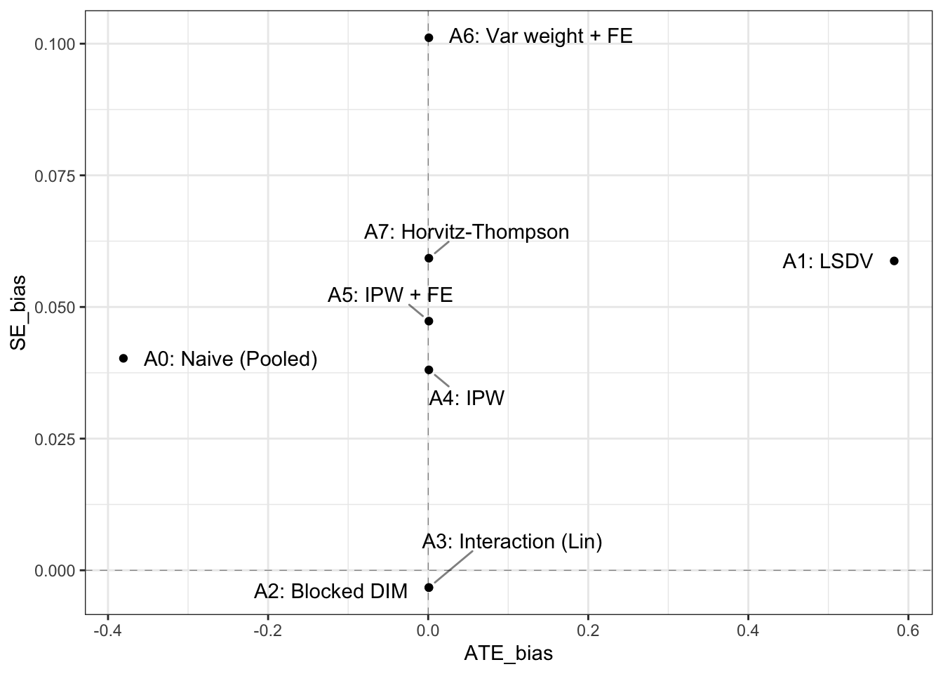

Interestingly, the largest differences between the approaches appear to arise from the way in which they calculate the standard error. A great thing about design diagnosis is that one can assess the performance not just of estimates but also of standard errors. We use standard errors as a measure of the standard deviation of the estimates under repeated experiments. This is a quantity we have access to from simulation and so for each approach we can compare the estimated standard error to the standard deviation of the sampling distribution of effects.

We see that many approaches appear overly conservative – particularly the weighting approaches, though one approach estimates, on average, a standard error that is marginally smaller than the real standard deviation of the sampling distribution of estimated effects.

In terms of estimates, however, there are no real differences in performance between approaches 2-9. The block-specific difference-in-means approach has the merit of conceptual simplicity and great performance. The IPW and Horvitz-Thompson approaches have the advantage that they can be used even if the heterogeneity in assignment propensities is at the unit-level, and not at the block-level. And regression-based approaches have the merit of making it simple to condition on available covariates.

This issue is surprisingly common

Many designs face this issue, where assignment propensities are different in different groups. Often the issue might not be immediately apparent. Some examples:

Subjects are randomly matched to play a game and you are interested in assessing the difference in play between single gender and mixed gender pairings. There are different numbers of men and women in the group.
A random set of children in a school are given some treatment and you are interested in seeing the effects on siblings of having another sibling treated. Families are of different sizes.
One village in each parish is selected for a treatment. But parishes are of different sizes.

In all these cases there is what looks at first glance to be equal assignment propensities across units but on closer inspection assignment propensities in fact depend on group size in some way.

See Gibbons, Serrato, and Urbancic (2018) for many examples in economics research and assessments of the implications of ignoring this issue.

References

Angrist, Joshua D. 1998. “Estimating the Labor Market Impact of Voluntary Military Service Using Social Security Data on Military Applicants.” Econometrica 66 (2): 249–88.

Gibbons, Charles E, Juan Carlos Suárez Serrato, and Michael B Urbancic. 2018. “Broken or Fixed Effects?” Journal of Econometric Methods.

Lin, Winston. 2013. “Agnostic Notes on Regression Adjustments to Experimental Data: Reexamining Freedman’s Critique.” The Annals of Applied Statistics 7 (1): 295–318.

Footnotes

This is a well known problem. See, for instance, Angrist (1998).↩︎
Functions in DeclareDesign create functions that take dataframes and return dataframes or statistics. Thus, we could also have taken one draw of the data using one_draw <- U() %>% Y %>% Z %>% R. The first five variables were created by U(): block indicates the block to which the unit belongs, prob indicates the probability of assignment to treatment, tau indicates the block-level treatment effect, indiv indicates the individual ID, and e is the error term. The function Y() appends the potential outcomes, Y_Z_0 and Y_Z_1, by taking e and adding tau in treatment. The function Z() appends two variables: Z is a vector of treatment assignments, block-randomized as a function of the block probabilities, while Z_cond_prob indicates the probability that a given unit is observed in the condition to which they were actually assigned. R() reveals the potential outcomes corresponding to the assignment.↩︎