An obvious requirement of a good research design is that the question it seeks to answer does in fact have an answer, at least under plausible models of the world. But we can sometimes get quite far along a research path without being conscious that the questions we ask do not have answers and the answers we get are answering different questions.

How could a question not have an answer? These situations can arise when inquiries depend on variables that do not exist or are undefined for some units. In this post, we’ll look at one way a question might not have an answer, but there are others.

Consider an audit experiment that seeks to assess the effects of an email from a person indicating that they are a Democrat (versus not revealing their party identification) on whether and how well election officials respond to requests for information. Whether or not a response is sent is easily observed and measured. The quality of the response is harder to measure, though some aspects, like the tone of the response, can be measured by human coders or possibly computers if fed enough training data.

More difficult than the measurement problem, though, is the problem of the “tone” of responses never sent. Simply dropping such observations is no good, because of the possibility that some officials would have responded in one condition but not in the other. After all, a main purpose of audit experiments is to measure the average effect of treatment on response rates, which requires believing that at least some officials would respond in one condition but not another.

For that kind of subject (so called if-treated or if-untreated responders), the effect of treatment on the tone of their email is undefined. It doesn’t exist. The question, “what is the effect of treatment on tone” has no answer if, in either the treatment or control condition, the subject wouldn’t respond. That question is only well-defined for subjects who always respond, regardless of treatment.

To summarize:

If treatment affects whether or not a subject responds, then the treatment effect on tone is undefined.
The average treatment effect (ATE) of treatment on tone is also undefined, because that estimand averages over all subjects.
The conditional average treatment effect (CATE) of treatment among “Always-responders” is well-defined.

Design delaration in words

Here are the key parts of the design:

Model: The model has two outcome variables, \(R_i\) and \(Y_i\). \(R_i\) stands for “response” and is equal to 1 if a response is sent, and 0 otherwise. \(Y_i\) is the tone of the response, which we’ll measure on a 1-7 “friendliness” scale. \(Z_i\) is the treatment indicator and equals 1 if the email indicates the sender is a Democrat and 0 otherwise. The table below describes four possible types of subjects who differ in terms of the potential outcomes of \(R_i\).
- Always-responders (ARs) always respond, regardless of treatment
- If-untreated responders (IURs) respond if and only if they are not treated
- If-treated responders (ITRs) respond if and only if they are treated
- Never-responders (NRs) never respond, regardless of treatment

The table also includes columns for the potential outcomes of \(Y_i\), showing which potential outcome subjects would express depending on their type. The key thing to note is that for all types except Always-responders, the effect of treatment on \(Y_i\) is undefined because messages never sent have no tone.¹ The last (and very important) feature of our model is that the outcomes \(Y_i\) are possibly correlated with subject type. Even though both \(E[Y_i(1) | \text{Type} = AR]\) and \(E[Y_i(1) | \text{Type} = ITR]\) exist, there’s no reason to expect that they are the same.

Causal Types
Type	\(R_i(0)\)	\(R_i(1)\)	\(Y_i(0)\)	\(Y_i(1)\)
Always-responders (ARs)	1	1	\(Y_i(0)\)	\(Y_i(1)\)
If-untreated responders (IURs)	1	0	\(Y_i(0)\)	NA
If-treated responders (ITRs)	0	1	NA	\(Y_i(1)\)
Never-responders (NRs)	0	0	NA	NA

Inquiry: We have two inquiries. The first is straightforward: \(E[R_i(1) - R_i(0)]\) is the Average Treatment Effect on response. The second inquiry is the undefined inquiry that does not have an answer: \(E[Y_i(1) - Y_i(0)]\). We will also consider a third inquiry, which is defined: \(E[Y_i(1) - Y_i(0) | \text{Type} = AR]\), which is the average effect of treatment on tone among Always-Responders.
Data strategy: The data strategy will be to use complete random assignment to assign 250 of 500 units to treatment.
Answer strategy: We’ll try to answer all three inquiries with the difference-in-means estimator.

This design can be declared formally like this:

design <-
# M: Model ----------------------------------------------------------------
  declare_model(
    N = 500,
    noise = rnorm(N),
    type = sample(1:4, N, replace = TRUE),
    AR = type == 1,
    IUR = type == 2,
    ITR = type == 3,
    NR = type == 4,
    
    # potential outcomes
    # AR and IUR types report in the control condition
    R_Z_0 = AR | IUR,
    # R and ITR types report in the treatment condition
    R_Z_1 = AR | ITR,
    # In control, ARs and IURs have different outcomes
    Y_Z_0 = ifelse(R_Z_0, as.numeric(draw_likert(-0.50 * IUR + noise)), NA),
    # In treatment, ARs and ITRs have different outcomes, and AR outcomes are higher
    Y_Z_1 = ifelse(R_Z_1, as.numeric(draw_likert(-0.25 * ITR + noise + 0.25)), NA)
  ) +
  
# I: Inquiry --------------------------------------------------------------
  declare_inquiry(
    ATE_R = mean(R_Z_1 - R_Z_0),
    ATE_Y = mean(Y_Z_1 - Y_Z_0),
    CATE_Y_AR = mean(Y_Z_1[AR] - Y_Z_0[AR])
  ) +
  
# D: Data Strategy --------------------------------------------------------
  declare_assignment(Z = complete_ra(N)) +
  declare_measurement(R = reveal_outcomes(R ~ Z),
                      Y = reveal_outcomes(Y ~ Z)) +
# Answer Strategy ---------------------------------------------------------
  declare_estimator(R ~ Z, inquiry = "ATE_R", label = "DIM_R") +
  declare_estimator(
    Y ~ Z, inquiry = list("ATE_Y", "CATE_Y_AR"), label = "DIM_Y")

Simulations

Here we simulate the design, diagnose, and plot the resulting output.

simulations <- simulate_design(design, sims = sims)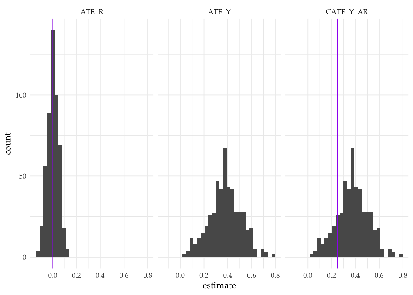

Design	Inquiry	Estimator	Outcome	Term	N Sims	Mean Estimate	Mean Estimand	Bias	Coverage	Power
design	ATE_R	DIM_R	R	Z	500	0.00	0.00	0.00	1.00	0.07
						(0.00)	(0.00)	(0.00)	(0.00)	(0.01)
design	ATE_Y	DIM_Y	Y	Z	500	0.38	NA	NA	NA	0.81
						(0.01)	NA	NA	NA	(0.01)
design	CATE_Y_AR	DIM_Y	Y	Z	500	0.38	0.25	0.13	0.85	0.81
						(0.01)	(0.00)	(0.01)	(0.02)	(0.01)

We learn three things from the design diagnosis.

First, as expected, our experiment is unbiased for the average treatment effect on response (ATE_R)
Second, our second inquiry (ATE_Y), as well as our diagnostics for it, are undefined. The diagnosis tells us that our definition of potential outcomes produces a definition problem for the estimand. Note that some diagnosands are defined, including power, but none of the diagnosands that depend on the value of the estimand (bias, coverage, rmse) can be calculated.
The third estimand (CATE_Y_AR) is defined but the estimator is biased. The reason is that we cannot tell from the data which types are the \(AR\) types; we are not conditioning on the correct subset. Indeed, we are unable to do so. If a subject responds in the treatment group, we don’t know if she is a \(AR\) or a \(ITR\) type; in the control group, we can’t tell if a responder is an \(AR\) or an \(IUR\) type. Our difference-in-means estimator of the CATE on \(Y\) among \(AR\)s will be off whenever \(AR\)s have different outcomes from \(ITR\)s and \(IUR\)s.

There are some solutions to this problem. In some cases, the problem might be resolved by changing the inquiry. Closely related estimands can often be defined, perhaps by redefining \(Y\) (e.g., emails never sent have a tone of zero). See Coppock (2019) for a more detailed discussion of solutions that may work for different research scenarios.

Some designs have badly posed questions and design diagnosis can alert you to the problem

Design delaration in words

Simulations

Other instances of this problem

References

Footnotes